CS224W Review
Pictures from: cs224w.stanford.edu
Not important: Lectures 1, 5, 9, 12, and 14.
Important: 2,4,6,7,8,10,11,13
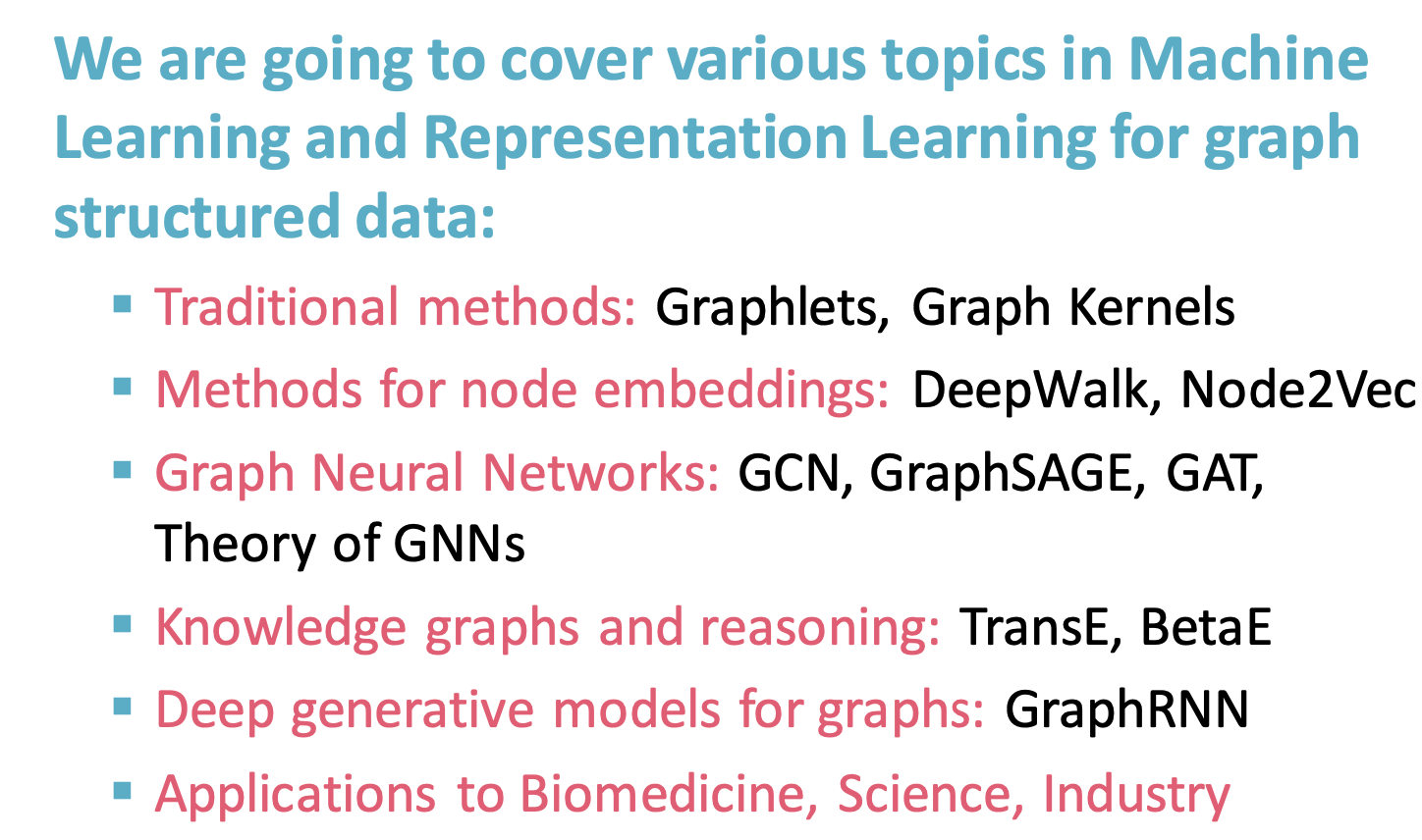
Topic list (not exhaustive):
- Centrality measures & PageRank
- ‼️GNN model & design space (message passing, aggregate, and combine) - core to build GNN
- knowledge graph embeddings, Query2Box, recommender systems(LightGCN), generative models
Lec1: Intro
Graph Intro
- picture: grid; NLP: sequences
- representation Learning:
- automatically learn the feature of graph
- similar nodes in the graph are embedded close together
- Course Outline:
- Graph ML tasks
- node classification
- link prediction
- Graph classification
- Clustering
- Edge-level task:
- recommender system
- node: user, items
- edge: user-item interactions
- PinSage:
- Node ???, edge ???
- Drug Side Effect: given a pair of drugs predict adverse side effects
- Node: drugs and proteins
- Edges: Interactions (different type edge, different side effect)
- recommender system
- Graph level task:
- Drug discovery: node-atoms; edges: chemical bonds
- physical simulation
- Graph Types:
- directed & undirected graphs
- directed graph node average degree: The (total) degree of a node is the sum of in- and out-degrees.
- heterogeneous graphs: different types of node and edge
- Biparitie graph:
- Folded networks: biparitie graph => projection
- weighted / un-weighted
- self-edges
- Multigraph: multi-edges between two nodes
- directed & undirected graphs
- adjacent matrix / Adjacent list
- Connectivity
- conneted graph
- unconnected-graph: adjacency matrix is block diagonal
- Strongly connected directed graph
- every node A, B, exist a path from A-B and B-A
- Weakly connected directed graph
- conneted graph
Lec2: Traditional ML
Traditional Methods for Graph ML
Traditional ML pipeline uses hand-designed features
node level:
node level features
Node degree
Node centrality: takes node importance in a graph into account
- eigenvector centrality
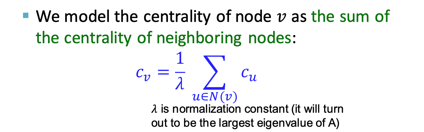
- centralitiy
is eigenvector of ,use largest eigenvalue and the corresponding
- Betweenness centrality
- A node is important if it lies on many shortest paths between other nodes.
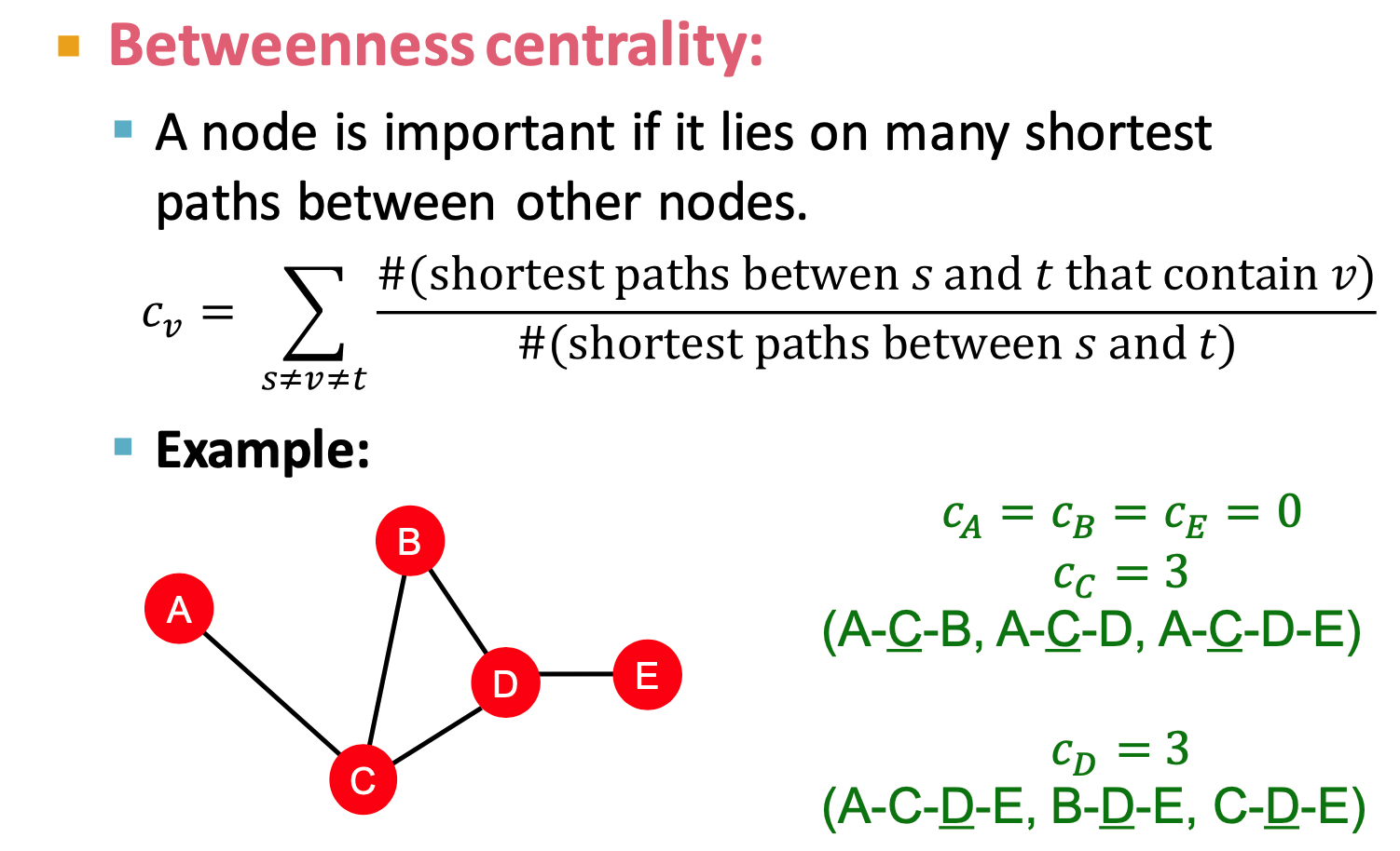
- at least 3 hop path ???
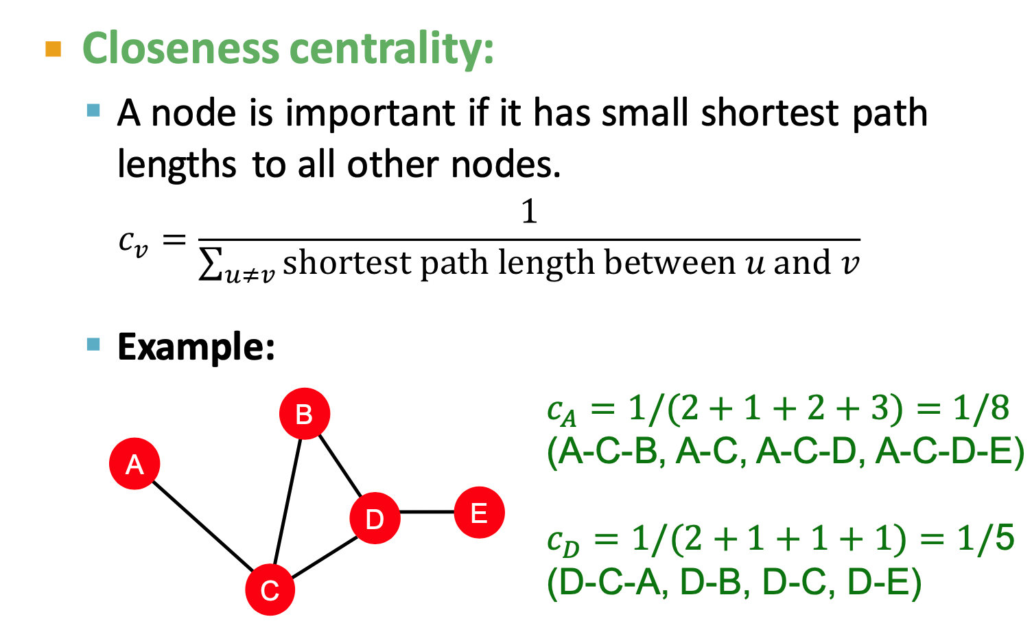
- Closeness centrality
- eigenvector centrality
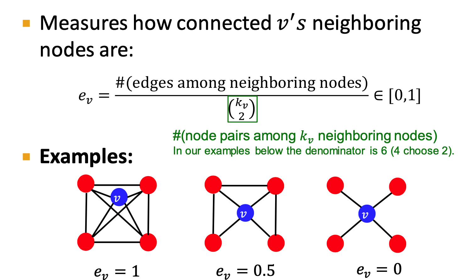
Clustering coefficient
- counts #(triangles)
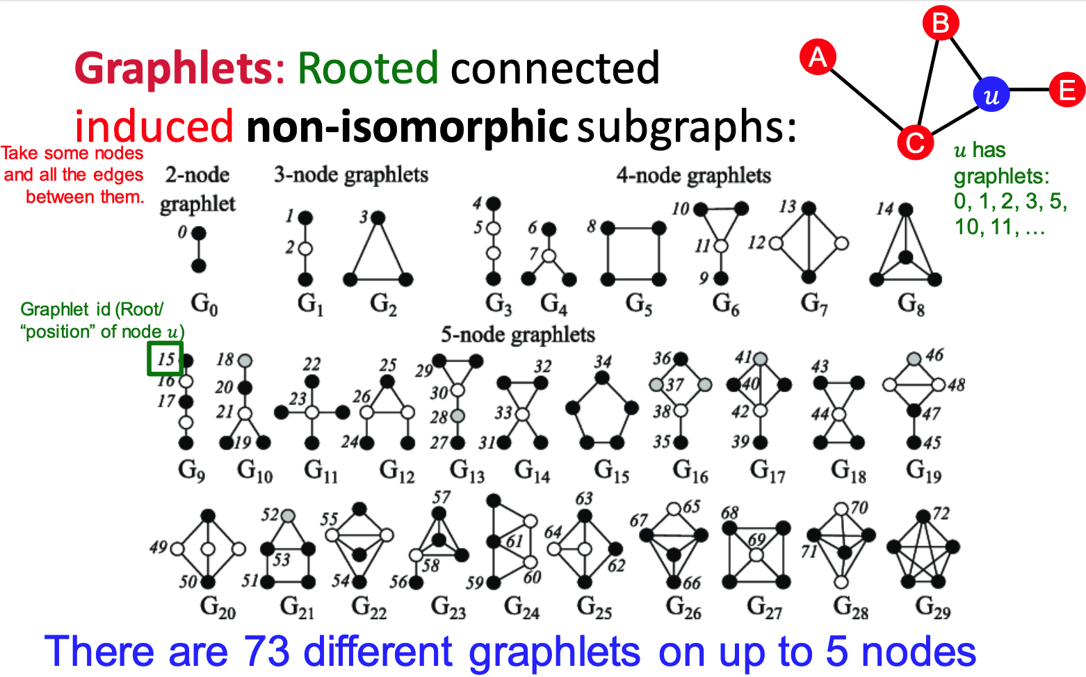
Graphlets:
- Rooted connected induced non-isomorphic subgraphs
- small subgraphs describe the structure of node
's neighborhood - GDV: graph degree vector
- #(graphlets) a node touches
- induced Subgraph: all the edges an
- isomorphism: same number of nodes; bijective mapping
important based features: predict influential nodes in a graph
Structure-based features: predict role a node plays
link prediction task and features
key: design features for a pair of nodes
link prediction task:
- links missing at random
- links over time
link prediction methodology:
- for each pair (x,y), compute score
- for each pair (x,y), compute score
Link-level features
- distance based featrue
- shortest-path distance between two nodes
- local neighborhood overlap
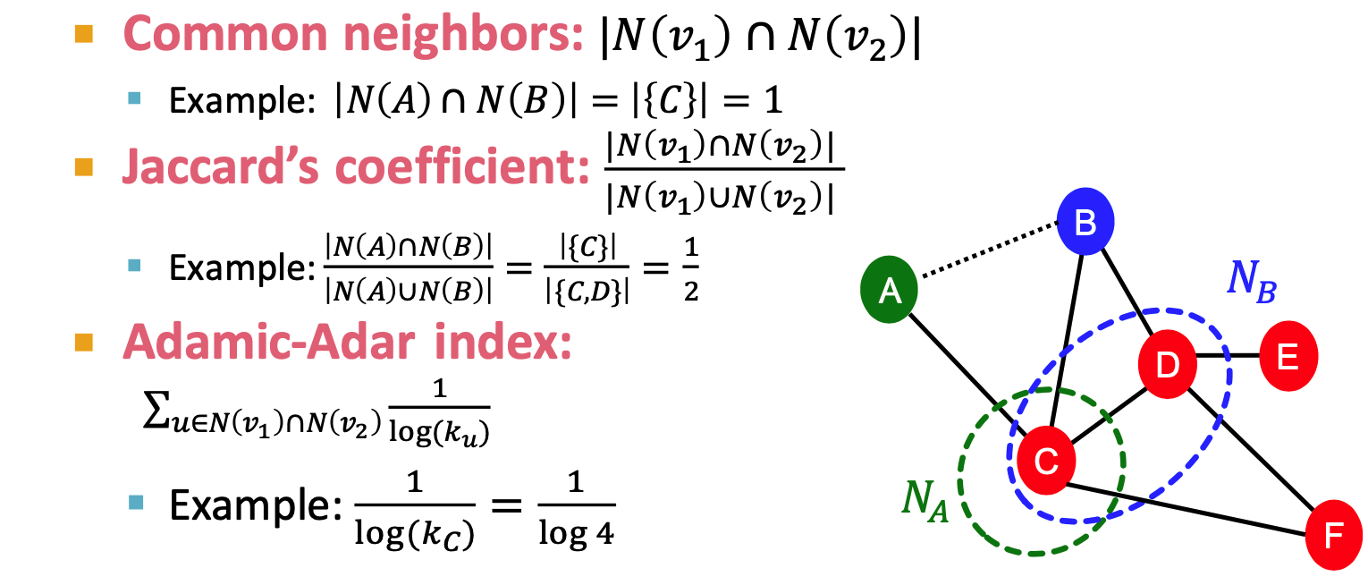
- limitation: metric is always zero if the two nodes do not have any neighbots in common
- global neighborhood overlap
(length K) - use
= #walks of length l - Katz index: number of walks of alll lengths between a given pair of nodes.
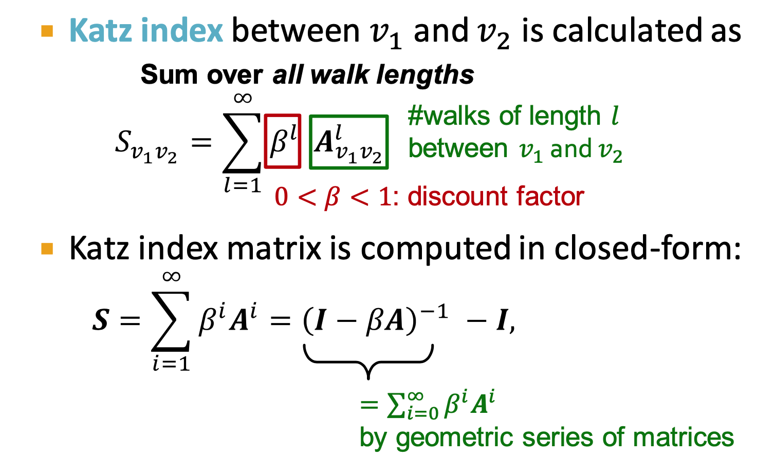
, score for node pair
- distance based featrue
Graph-level Features
kernel methods
- design kernels instead of feature vectors
semidefinite , is a feature representation (Graph feature vector) - Bag-of-Words for a graph
Graphlet Kernel
Graphlet (different definition): not need to be connected; not rooted
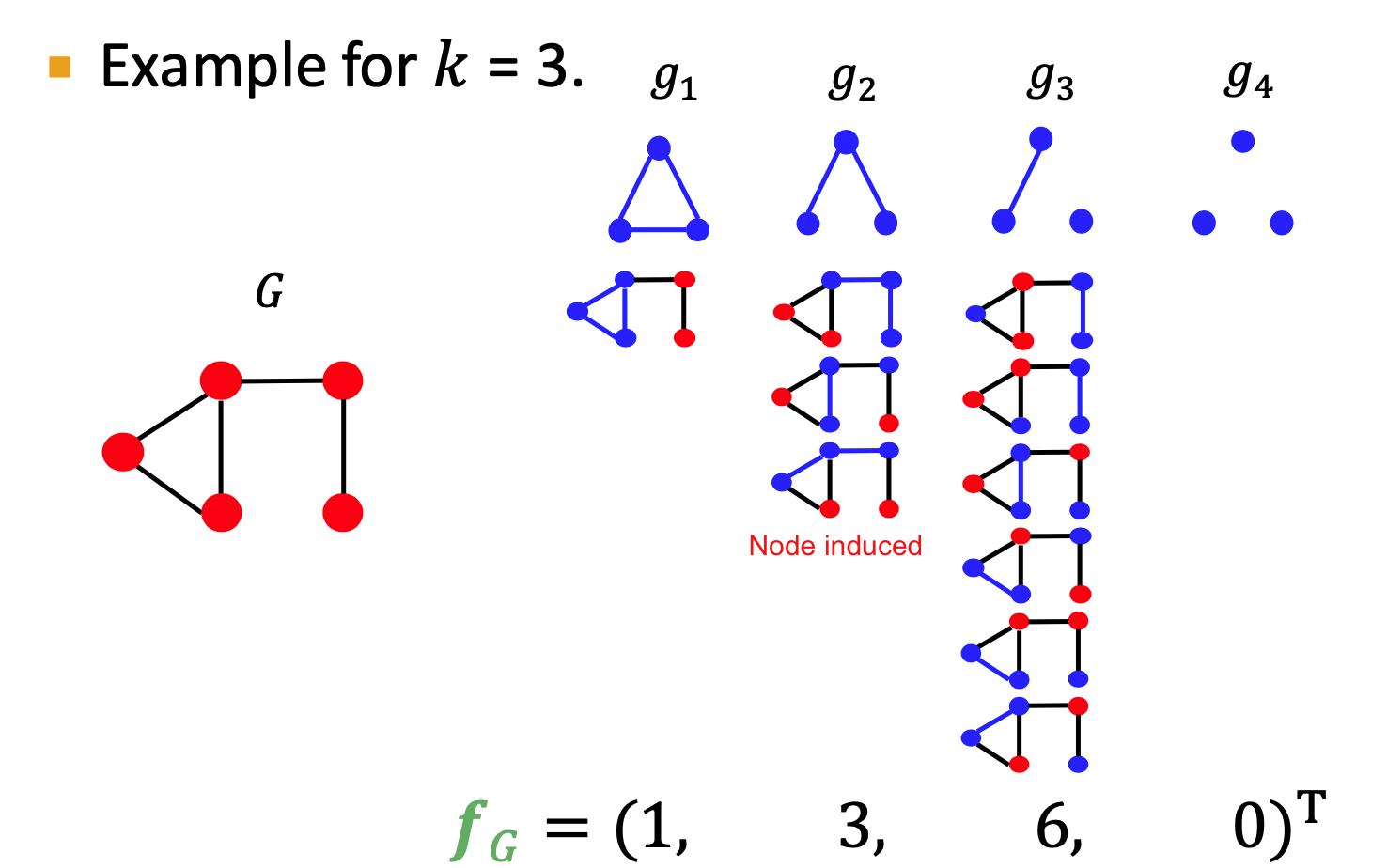
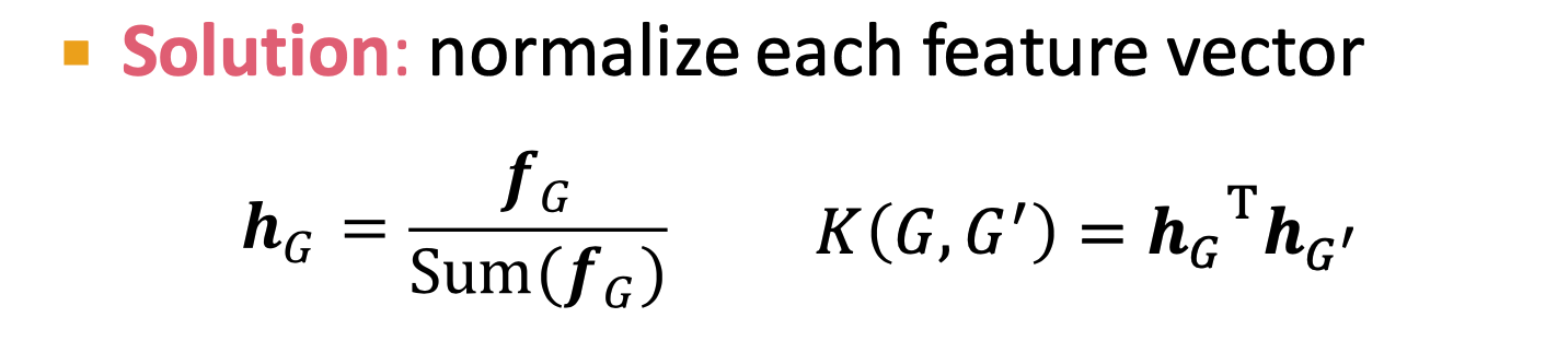
normalize
Weisfeiler-Lehman Kernel
- use neighborhood structure to iteratively enrich node vocabulary
- Color Refinement
- HASH function:(current node, neighbor nodes)
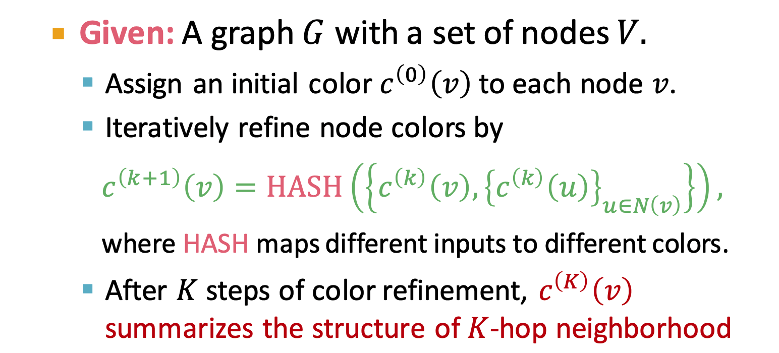
- total time complexity is linear in #(edges)
Lec3: Representation Learning
Node Embeddings
- Graph Representation Learning
- task-independent feature learning for machine leanring with Graphs
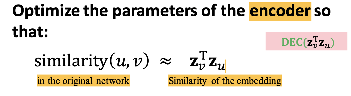
Encoder and Decoder
Goal: similarity in the embedding space (e.g., dot product) pproximates similarity in the graph
Three important things need to define:
- similarity
- a measure of similarity in the original network
- Encoder
- nodes to embeddings
- Decoder
- map from embeddings to the similarity score;
- Decoder based on node similarity
- maximize
for (u,v) who are similar - how to define similar?
- similarity
shallow encoding
is the matrix to optimize; v is indicator vector(all zeroes except a one in column indicating node v) - encoder is just a embedding-lookup
- Shallow: each node is assigned a unique embedding vector
- directly optimize the embedding of each node
- Substitue method/Deep encoders(GNNs): DeepWalk, node2vec ????
key: define node similarity (can use )
Unsupervised/self-supervised learning embeddings
Random Walk Approches for node Embeddings
Random Walk => define node similarity (Decoder)
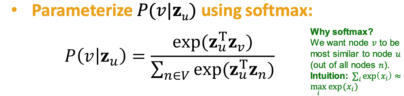
Probability
: predicted probability of visiting node on random wals starting from node is the embedding of node , our target - Non-linear functions used to produce predicted P
- Softmax: turn K real values into K probabilities that sum to 1
- Sigmoid
Random walk:
Is it a definiation of similarity
If
and co-occur on a random walk, is similar; high-order multi-hop information - incorporates both local and high-order neighborhood information
the probability that u and v co-appear on a random walk steps:
- use random walk to get
- optimize embedding to encode the
- use random walk to get
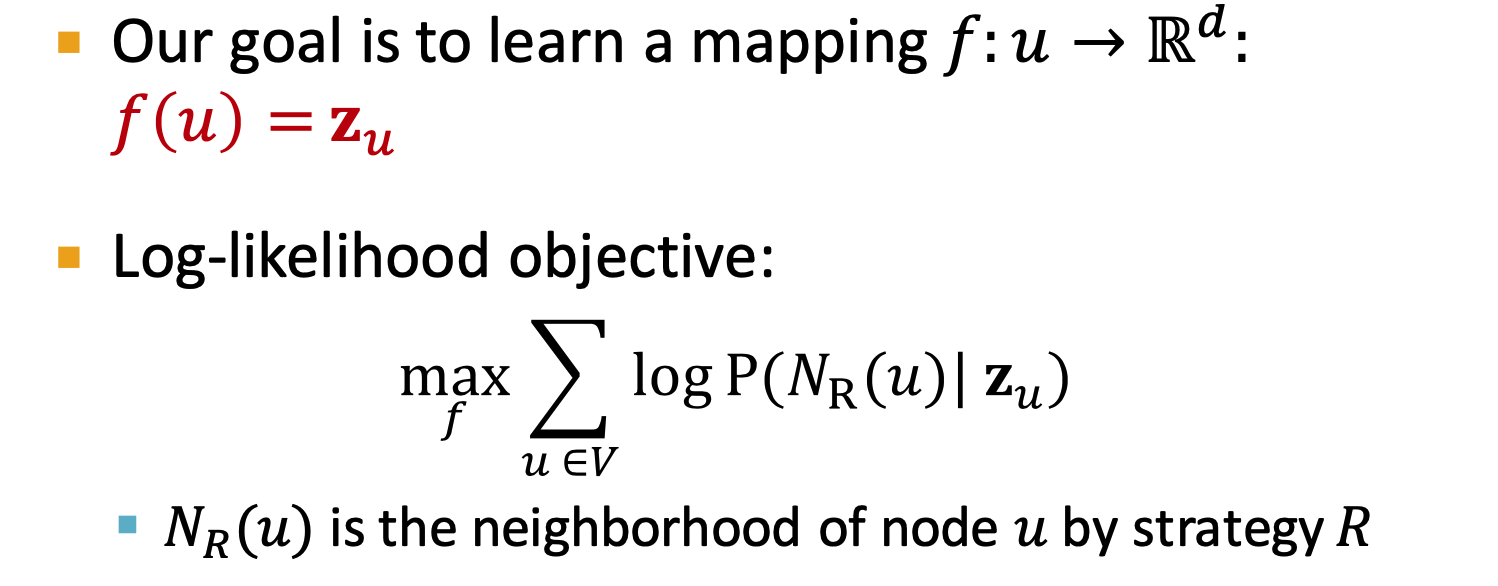
Unsupervised Feature Learning
- Learn node embedding such that nearby nodes are close together in the network
- nearby: random walk co-occurrance
- nearby nodes: neighborhood of
obtained by some random walk strategy
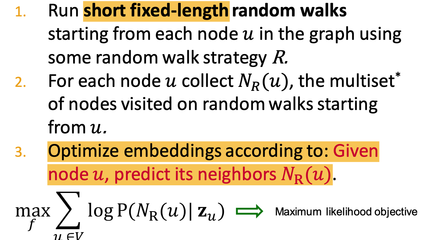
- As Optimization - Random Walk Optimization
- Steps:
- run short fixed-length random walks
- get multiset of nodes visited on random walks starting from
- Optimize embeddings according to predicted neighbors
- Learn node embedding such that nearby nodes are close together in the network
Optimization target of random walk

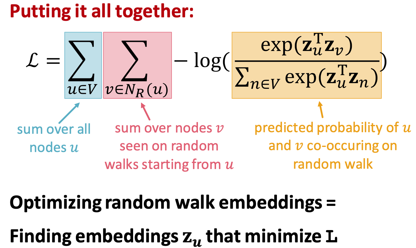
- Negtive sampling to approximate
- k random negtive samples
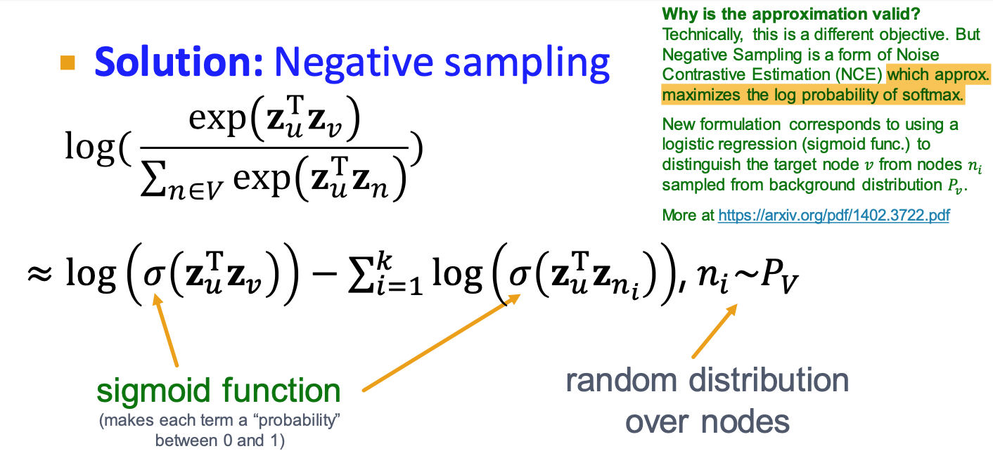
- Stochastic Gradient Descent: evaluate it for each individual training example
- k random negtive samples
How random walk
- Deepwalk: fixed-length, unbiased
- node2vec: biased 2nd order random walk
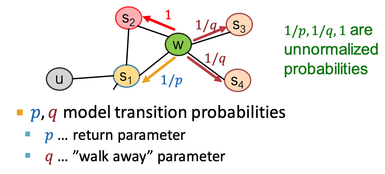
Node2vec: Biased Random walk
- trade off between local and global views
- BFS, DFS
- return parameters
: return to where it comes - in-out parameters
: ratio of BFS vs. DFS - BFS like: low
; DFS: low
Embedding Entire Graphs
Approach1: sum
Approach2: create a virtual node, and connect the node with each/every node in subgraph/total graph
Approch3: Anonymous Walk
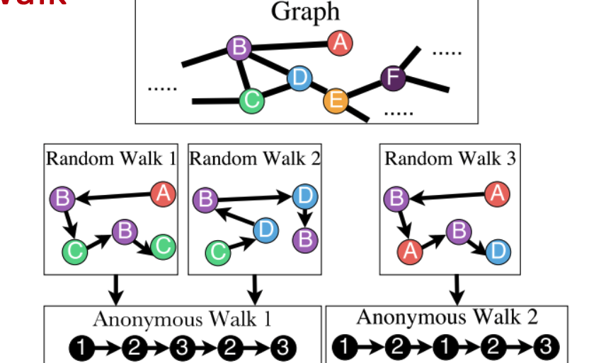
- States in anonymous walks correspond to the index of the first time we visited the node
- Represent the graph as a probability distribution over these walks.
Approach 3: Anonymous Walk Embeddings
Idea 1: Sample the anon. walks and represent the graph as fraction of times each anon walk occurs.
Idea 2: Learn graph embedding together with anonymous walk embeddings.
Lec4: Graph as Matrix
Outline:
- Determine node importance via random walk (PageRank)
- stochastic matrix M
- Obtain node embeddings via matrix factorization (MF)
- View other node embeddings (e.g. Node2Vec) as MF
PageRank
flow model:
- If page i with importance
has out-links, each link gets votes
- If page i with importance
Stochastic adjacency matrix M (column stochastic)
- ‼️ ji not ij
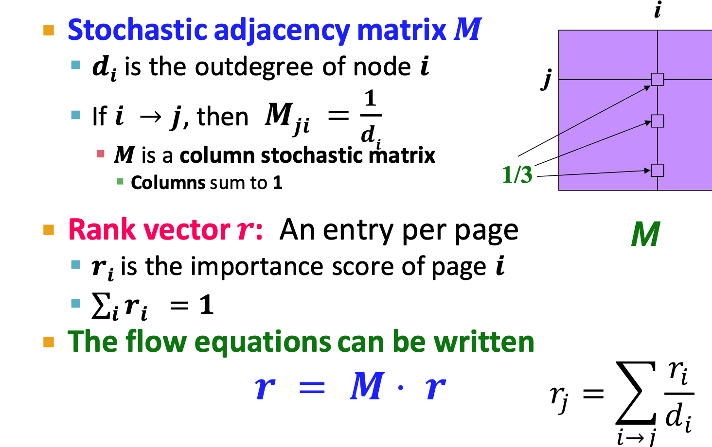
- flow equation: r=Mr
- stationary distribution
- rank vector
is an eigenvector of the column stochastic matrix (with eigenvalue 1)
- ‼️ ji not ij
Solve PageRank
Power iteration:
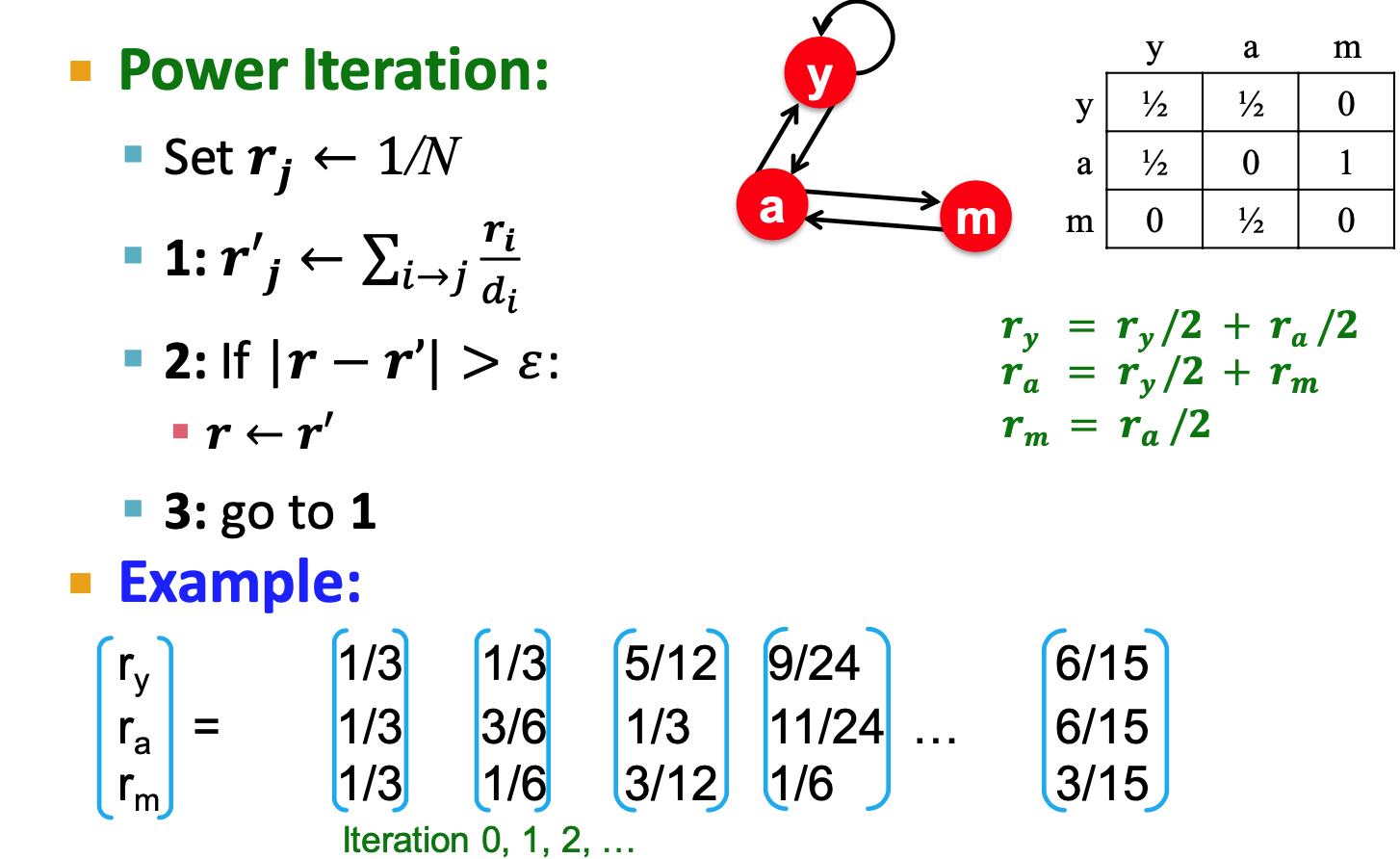
Use last iteration value?
problems:
- Dead ends;
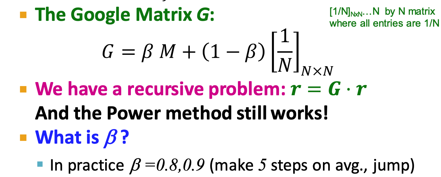
- Solution: teleport with prob.
- Dead ends ,with prob. 1.0 teleport
- Solution: teleport with prob.
- Spider traps: spider traps absorb all importance
- Dead ends;
PageRank
- each step:
- with prob.
, follow a link at random 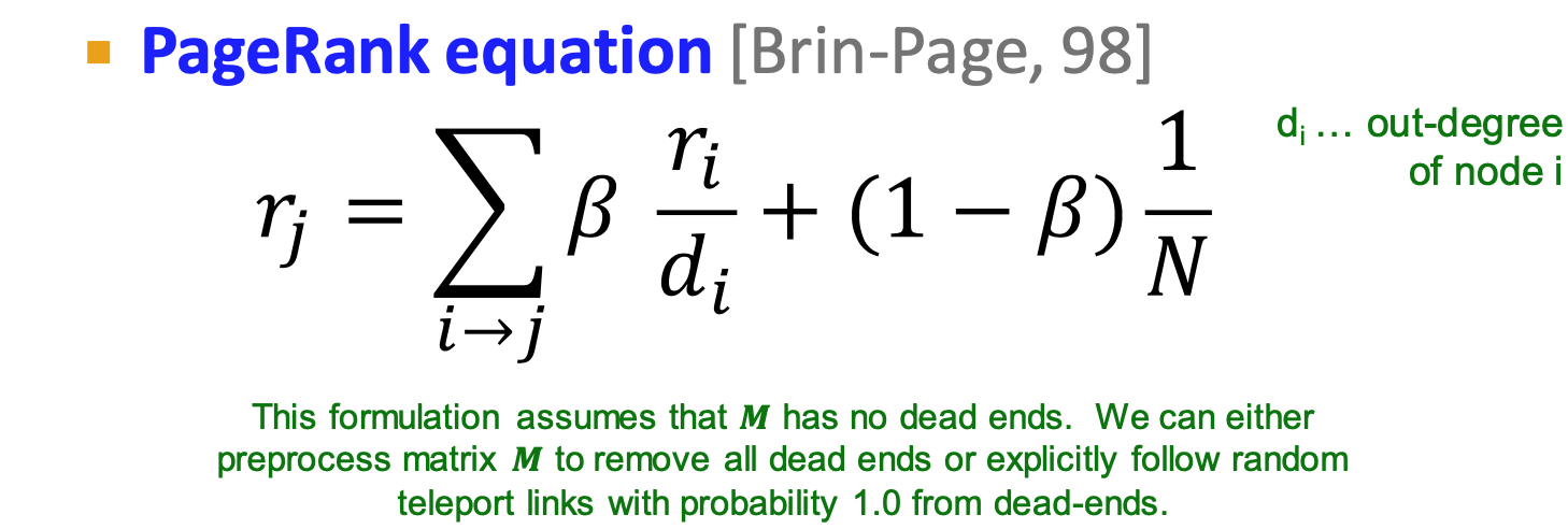
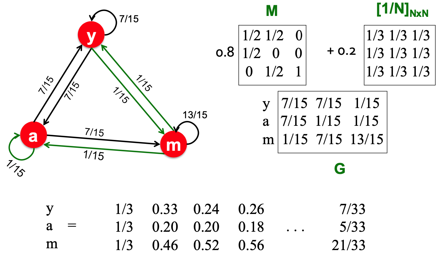
- with prob.
- each step:
Random walk with restarts and PPR
- PPR: Personalized PageRank
- Ranks proximity of nodes to the teleport nodes
(start nodes) - eg, recommend related items to item Q, teleport could be {Q}
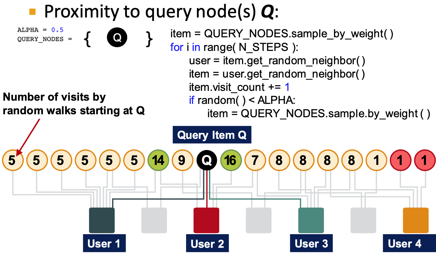
- Ranks proximity of nodes to the teleport nodes
- PageRank: teleport to any node, same probability
- Personalized PageRank: different landing probability of each node
- Random walk with restarts: always to the same node
- Random walk is to get the teleport nodes
Matrix Factorization
Matrix Factorization:
- get node embedings
- shallow embedding, ENC(v) =
; - similarity: node u, v are similar if they are connected by an edge
is generally not possible - learn
approximately - opptimize L2 norm
- learn
DeepWalk and node2vec have more complex node similarity - different complex matrix
limitations of MF and random walk
- Cannot obtain embeddings for nodes not in the training set
- Cannot capture structural similarity
- DeepWalk and node2vec do not capture structural similarity
- Cannot utilize node, edge and graph
- DeepWalk/node2vec embeddings do not incorporate node features
node embeddings based on random walks can be expressed as matrix factorization.
Lec5: Node Classification
Message Passing & Node classificaiton
not represent learning
collecitve classification: assigning labels to all the nodes in a network together
- correlations: homophily, influence
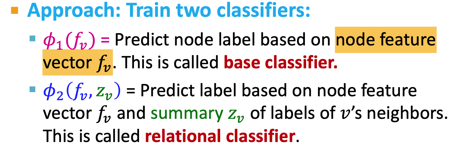
Methods:
- Relational classification
- Iterative classification
- Correct & Smooth
Relational Classification
idea: Propagate node labels across the network
steps:
- initialize unlabeled nodes
- initialize unlabeled nodes
Let
the posibility that node Yi belongs to class 1 Update each node one by one (use the new
) 
Limits:
- convergence is not guaranteed (use a maximum number of iterations)
- Model cannot use node feature information
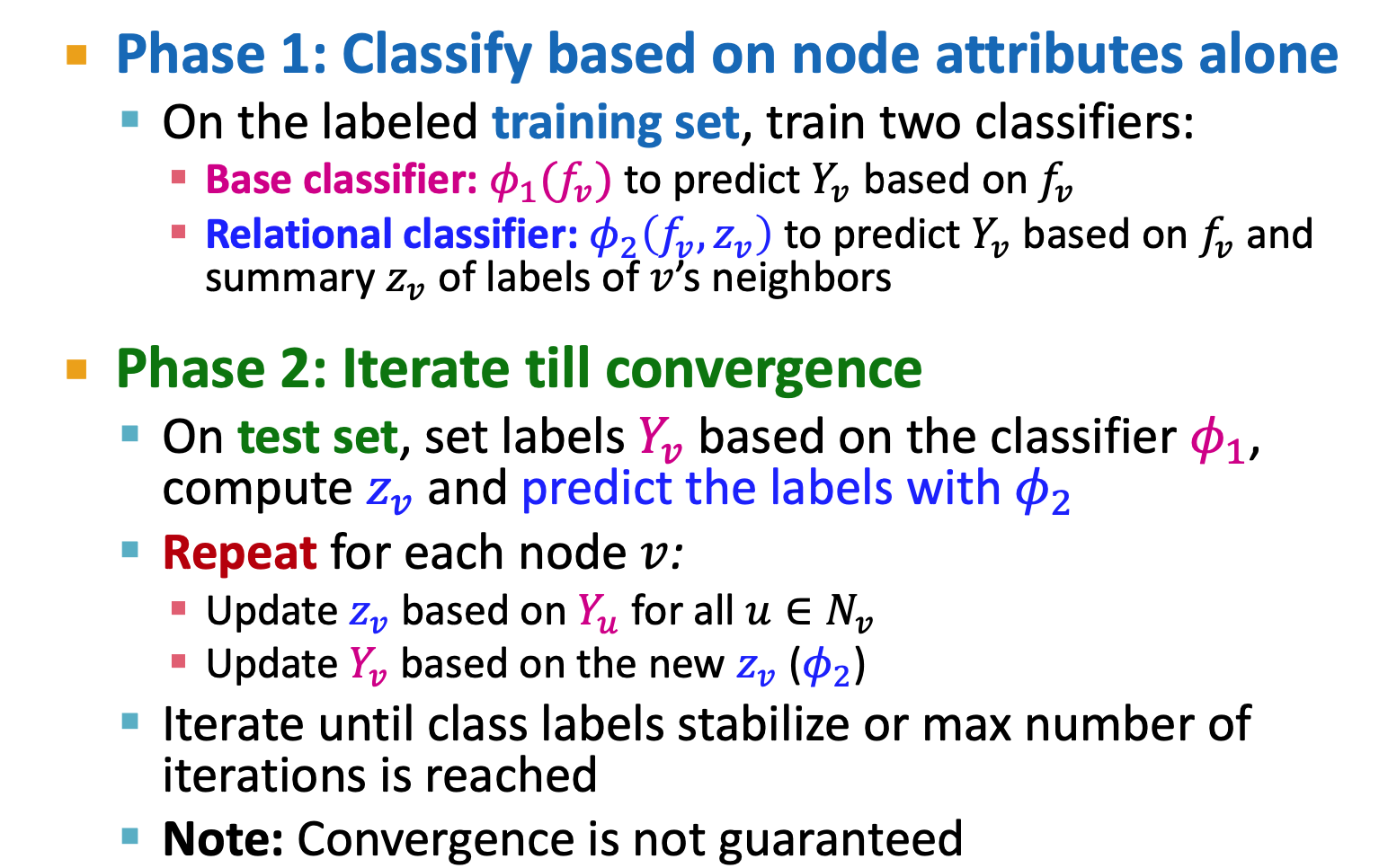
Iterative Classification
- relational classifier does not use node attributes
- iterative classifier: attributes and labels
could be: - histogram of the number/fraction of each label in
- most common label in
- Number of different labels in
could base on neighbors's label or neighbors' features could be incomplelete - could use -1 to denote
- If use
predict label, it wil bring wrong information to . We do not want to have wrong information.
- histogram of the number/fraction of each label in
- Only use
to initialize, and use to iterate (to update )
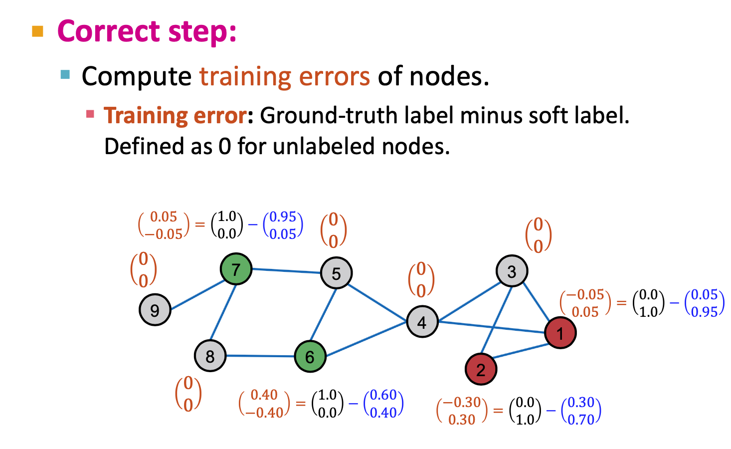
Correct & Smooth
- Train base predictor(Liner Model or MLP)
- Use the base predictor to predict soft labels of all nodes.
- Post-process the predictions using graph structure to obtain the final predictions of all nodes.(correct + smooth)
- step 1&2 =
- Correct step:
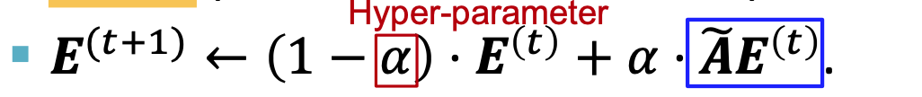
- Diffuse traingin error: same like pageRank/ Flow formulation
like a random walk distribute matrix diffusion matrix : 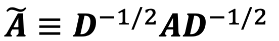
- A: adjacency matrix + self loop
- D = diag(d1, d2,.., dn)
- Smooth Step

- Smoothen the prediction of the base predictor (smoothen prediction with neighbors)
- Examples
- diffusion matrix
: - all the eigenvalues
are in [-1, 1] , eigenvector is 
- all the eigenvalues
Lec6 GNN
Graph neural Networks (Deep graph Encoders)
ENC(v) = GNN, can be combined with node similarity functions in Lec3
Basics of Deep Learning
ML = optimization
- Supervised Learning: (today's setup) input
, label - taget :
- Loss function: L2 function
- Don't care about the value of L, only care about
(variable parameters)
- Don't care about the value of L, only care about
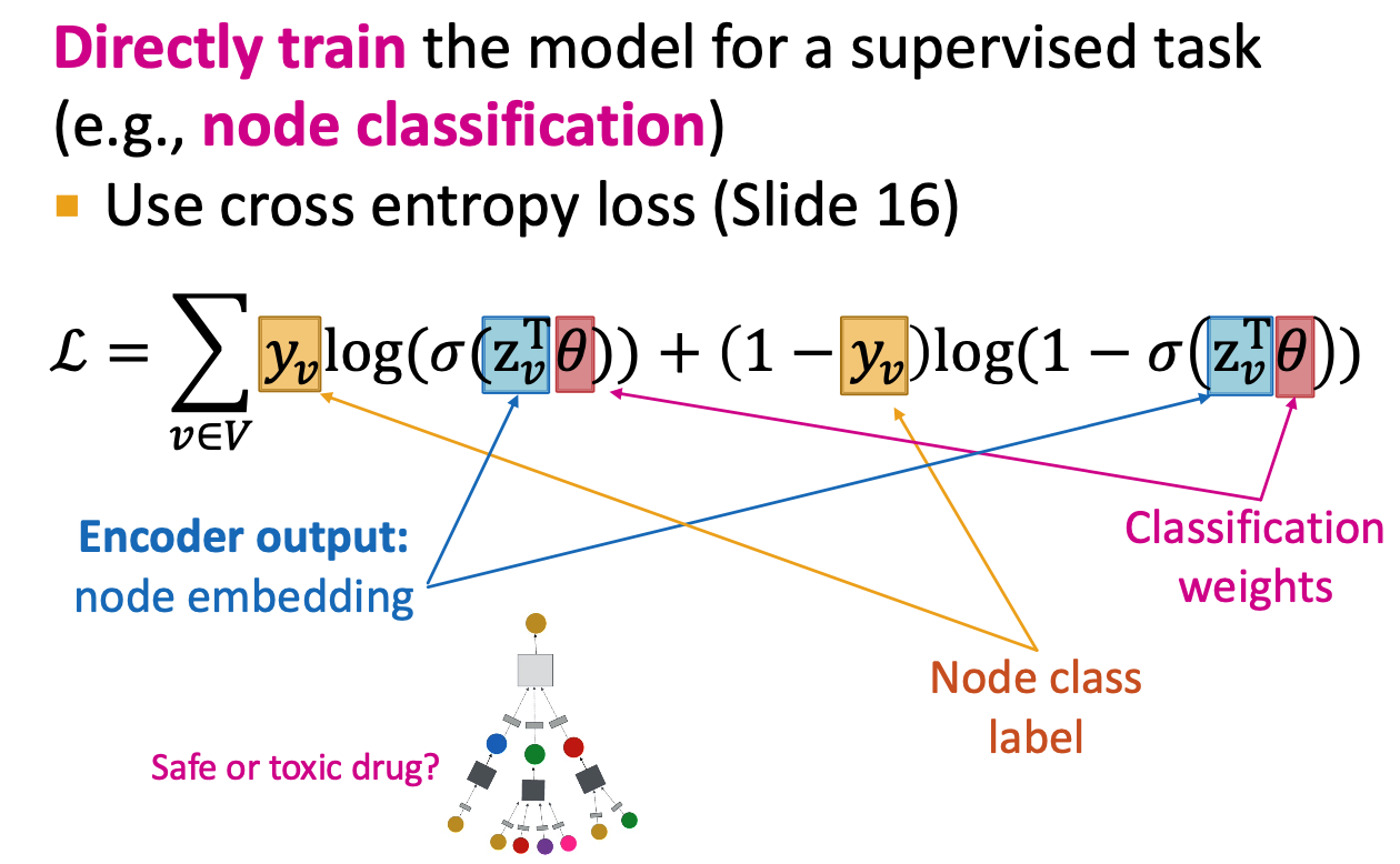
- Loss function Example: Cross Entropy(CE)
- the lower the loss, the closer the prediction is to one-hot
- Gradient vector/ Gradient Descent
- Gradient Descent is slow: need to calculate the entire dataset
- SGD: Stochastic Gradient Descent
- Minibatch
- Concepts: batch size; Iteration(on mini batch); Epoch(on the entire dataset)
- SGD is unbiased estimator of full gradient
- Back Propagation
- predefined building block functions
- each such 𝑔 we also have its derivative 𝑔′
- chain rule:

- Hidden Layer
- Forward propagation
- predefined building block functions
- Non-linearity
- ReLU
- Sigmoid
- MLP(Multi-layer Perceptron)
- bias vector can be write into
: add a dimision of , always be 1
- bias vector can be write into
Deep learning for graphs
A naive Apporach: use adjacent matrix
- limitation:
- too many parameters
- different size of graph
- sensitive ot node ordering
- limitation:
Convolutional Networks
For graph, Permutation Invariance
Different order plan, same result of
target: learn
who is permuation invariance node feature : permutation equivariance function GNN consist of multiple permutation equivariant / invariant functions
Equivariance and Invariance has a little difference
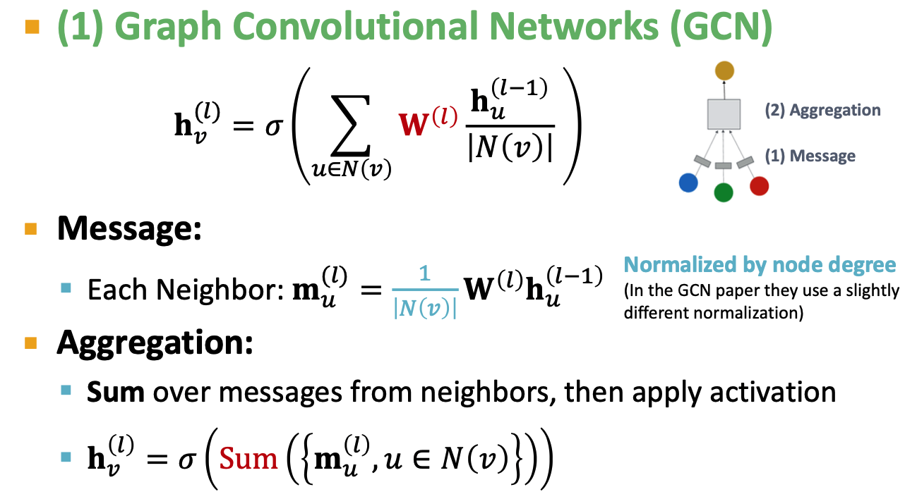
Graph Convolutional Networks
Output: Node embeddings/ subgraph embeddings/ graph embeddings
Node takes information from it's neighbors
Node's computation graph:
- every node defines a different computation graph
Deep Model: Many Layers
- a node can appear in multiple places
Neighborhood Aggregation
Basic approach: average neighbor messages and apply a nerual network

and is related to layer number Loss function:
- Parameters:
- Assume: parameter sharing ??? (maybe sharing
) - rewrite into matrix formulation

is sparse
- Parameters:
Unsupervised Training
- use network similarity to provide loss function / as the supervision
- Similar nodes have similar embeddings: Random walk, matrix factorization, node proximity

Supervised Training
- Use loss function like CE
- Steps:
- define a neigghborhood aggregation function
- Define a loss function on the embeddings
- Train on a set of nodes, i.e., a batch of compute graphs
- Generate embeddings for nodes as needed
- shared parameters
- Use loss function like CE
Inductive Capability
- Train on a graph A and collected data about organism B
- Train on part of nodes, generated node embedings on different nodes(never trained with)
- Because the
is shared - Create computational graph of a new node
- forward
- Because the
Difference of CNN and GNN
- CNN is not permutational equivariant

- Learn different
for different neighbor of pixel
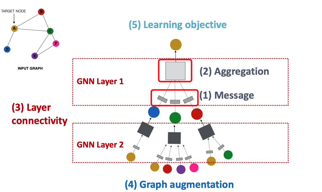
Lec7 General Perspective of GNN
Building blocks of GNN:
- message
- aggregation
- Layer connectivity
- Graph augmentation
- learning objective
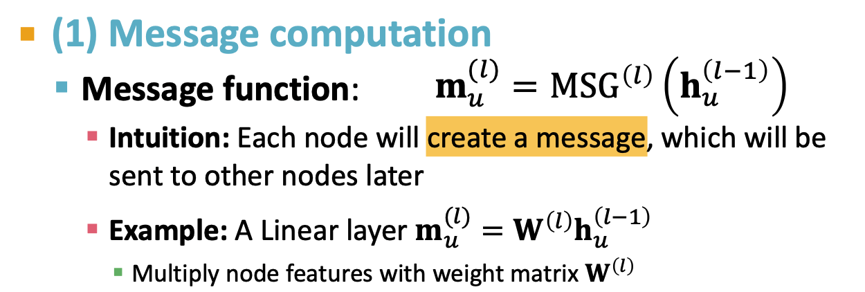
A single layer of GNN
message + aggregate
message:
Aggregation:
aggregate()is only for neighbors, can ignore self-loop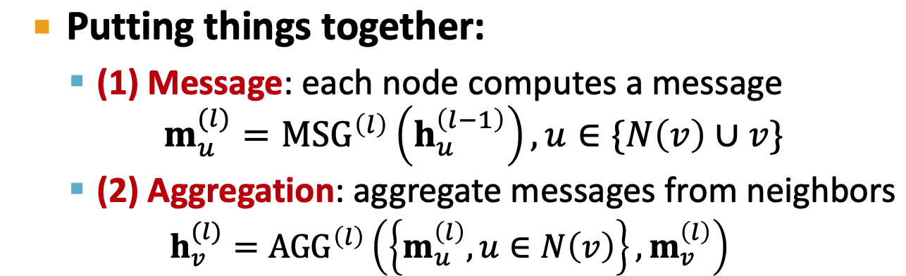
GCN: classical GNN layer
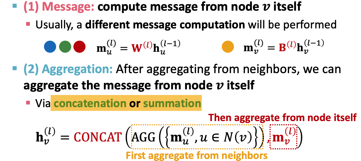
GraphSAGE:
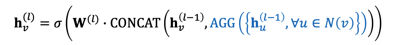
- Two stage aggregation
- aggregate neighbors
- aggregate over node itself
can be what? (In paper, different kinds of AGG), has to be differentiable - Mean
- Pool
- LSTM
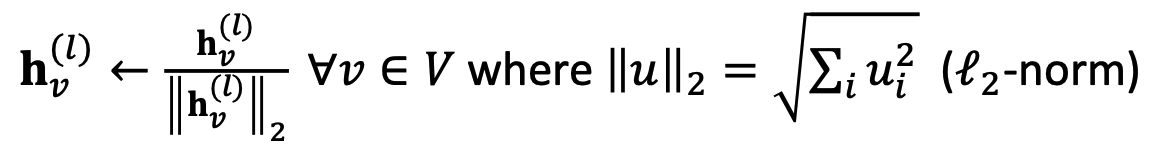
- L2 normalization: to every layer
GAT
In GCN,
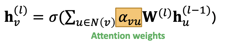
is 1/degree_v, GAT: make
learnable compute attention coefficients:
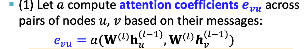
Nomorlize
using softmax What is a()?
- eg, a single layer NN
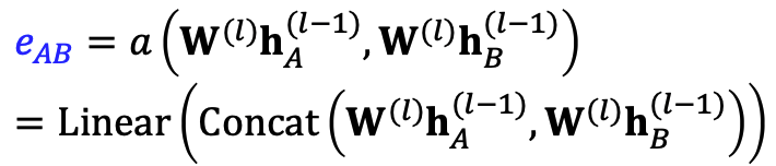
- The parameters are jointly learned
Multi-head attention: output are aggregated(concat or sum)
Batch Normalization
Dropout:
- use in linear layer of message function
Activation function/non linear
Stack GNN layers
- over-smoothing
- shared neighbors grow quickly
- adding more GNN layers do not always help
- Expressive power of shallow GNN
- Increase the layers in message & aggregation
- Add layers that do not pass messages
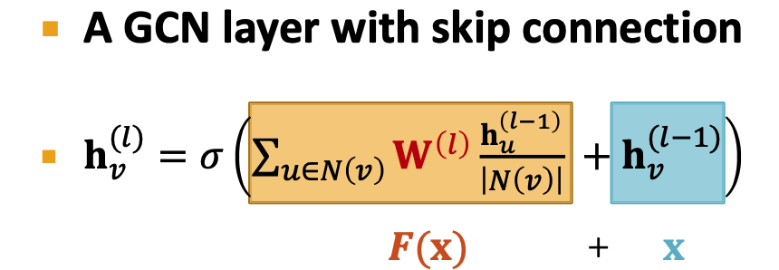
- Add skip connections
Graph Manipulation Approaches
Graph Freature manipulation
- feature augmentation
- assign constant node feature
- assign one-hot node feature
- Add traditional node feature/embedding
- feature augmentation
Graph Structure manipulation
too sparse: add virtual nodes/edges
- add virtual edges: use
instead of , use bipartite graphs - add virtual nodes: connect every node in graph
- add virtual edges: use
too dense: sample neighbors when message passing
- differ from drop out?
- neighborhood sampling is not random. Drop out is random ?
- drop out is for training; neighborhood sampling is for both training and testing
- Neighorhood sampling is not random sample
- but use random sampling to pick the most important neighbors
- sort the neighbors with visit count and pick top k
- differ from drop out?
too large: sample subgraph to comput embeddings
Lec8 Prediction
Prediction with GNNs
input graph => GNN => node embeddings => prediction head
- different task levels require different prediction heads
node level:
- directly make prediction using node embeddings
edge-level prediction
Head_edge could be:
concatenation + linear
dot product (only for 1-way prediction)
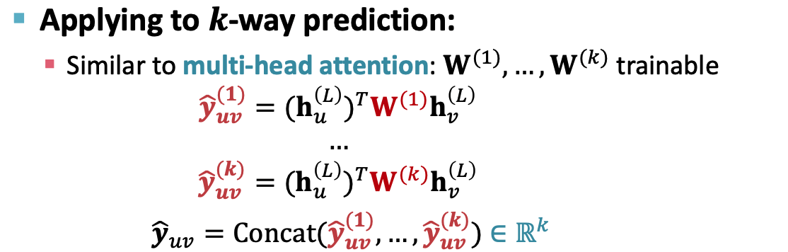
dot product for k-way prediction
Graph-level

- similar to AGG() in a GNN layer
- Head_graph could be:
- global mean pooling
- global max pooling
- global sum pooling
- global pooling will lost information
Hierarchical Global Pooling
- DiffPool
- GNN A: compute embeddings
- GNN B: compute the cluster taht a node belongs to
- DiffPool
GNN training
- supervised / unsupervised
- classification / regression
- classification loss: cross Entropy
- Regression loss: MSE loss
- Metrics for Binary Classification:
- Accuracy
- Precision
- Recall
- F1-score
- ROC curve/ROC AUC
Setting-up GNN prediction Tasks
- dataset split:
- Training seg
- validation set
- test set
- Solutions:
- Transductive setting: input graph can be observed in all the dataset;
- only split the node labels
- only comput loss on part of nodes
- Inductive setting: break the edges
- Transductive setting: input graph can be observed in all the dataset;
- Link Prediction task:
- We need to create the labels and dataset splits on our own
- hide some edges from the GNN
- Assign 2 types of edges in the original graph
- message ages for message passing
- supervision edges, take away, not the input to GNN
- calculate the loss on supervision edges
- Transductive
- 4 types of edges
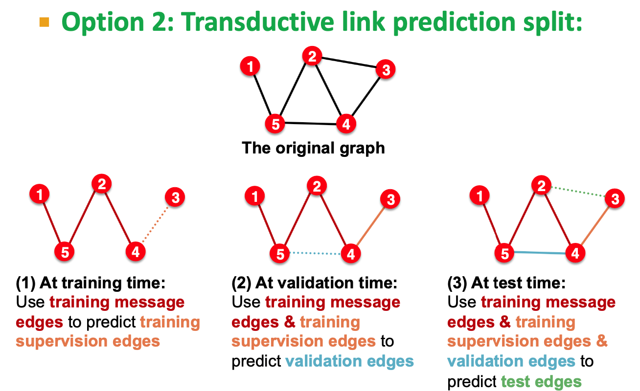
- => (2) => (3) view as time passing, it's very natural
Lec9 GNN Expressiveness
GCN(mean-pool): Element-wise mean pooling + linear + ReLU non-linearity
- GNN caputres local neighborhood structures using computational graph
- GNN only see node features in computational graph
- Can not distinguish:
- same computational graph
- same node feature
GraphSAGE(max-pool)
injective function: most expressive GNN model should map subtrees to the node embeddings injectively
- the most expressive GNN use injective function
- GNN can fully distinguish different subtree structures if every step of its neighbor aggregation is injective
- expressiveness depends on neighborhodd aggregation function
- GCN(element-wise mean-pool)
- GraphSAGE(element-wise max-pool)
Design injective function using neural network
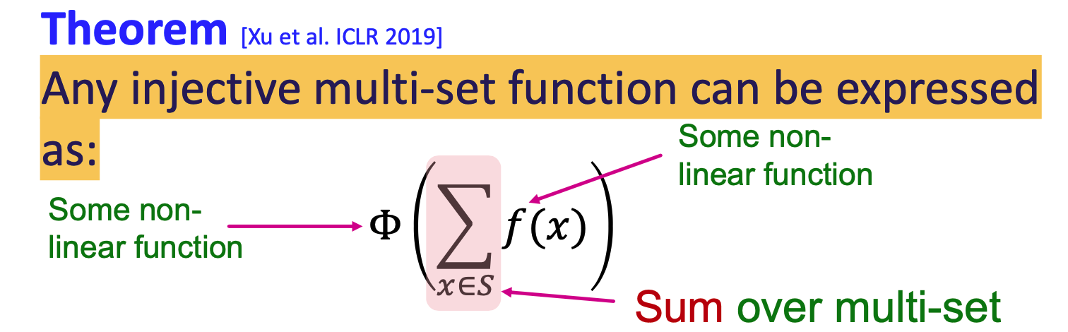
- use multi layer perceptron to approximate
- GIN(Graph Isomorphism Network):
- GIN uses a neural network to model the injective HASH function of WL kernel
- key is to use elment-wise sum pooling, not max/mean
## Lec10 KG Completion
- KG: l=0 is not a problem, h=t is a problem. h and t are not distinguishable
Heterogeneous Graph
multiple edges types and multiple node types
extend GCN to handle heterogeneous graph
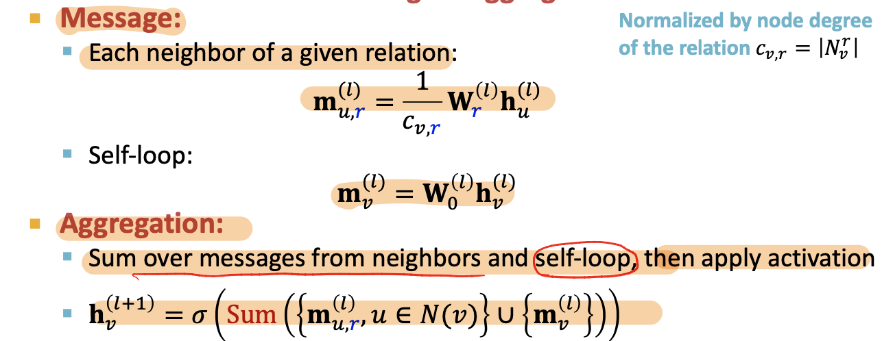
Relational GCN
aggragate using different relation type
color = different relation type

- over all the relation type, over all the neighbors
- Message:each neighbor of a given relation + self-loop
- Aggregation: Sum over messages from neighbors and self-loop, then apply activation
Scalability: (L layers of the computational graph)
- Each relation has L matices:
- A lot of parameters -> overfitting issue
- Two methods to regularize the weights
[avoid too much parameters and overfitting] - use block diagonal matirces
- Basis / Dictionary learning
- Each relation has L matices:
Block Diagnoal Matrices
make the weights sparse
B low dimensional-matrices, then # param reduces from
to
Basis Learning:
- Share weights across different relations
, a_rb is for each relation, and V_b is shared for all relations - only needs to learn
- only need to learn B scalars
- only needs to learn
- B group of similar relations, within a group, the relation share
Eg, node classification with RGCN
- use the representation of the final layer
represent the probability of that class
- use the representation of the final layer
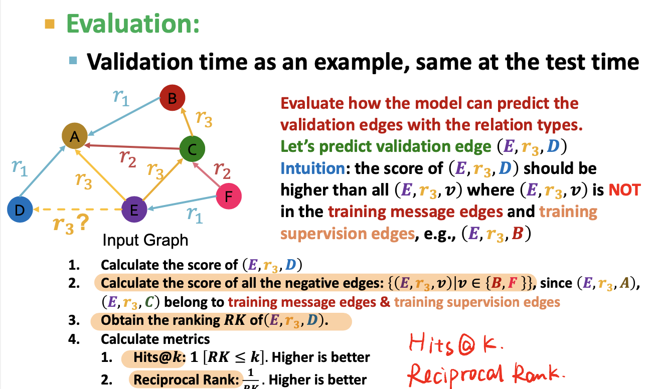
Eg: link predicition with RGCN, what kind of relation
- (E,r3,A), input is the final layer of E and A,
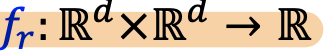
- use a relation-specific score function
- use negive sampling
- Training supervision edge / Traning message edges
- negtive edge: actually does not exsit
- not belongs to exsiting edges
- exsiting edges = training message edges & training supervision edges
- Maximize the score of training supervision edge
- Minimize the score of negtive edges
- validation edge: not visible when training
- training message edges & training supervision edges: all existing edges
- Evaluation:
- Metrics:
- Hits@k
- Reciprocal Rank
- Become a ranking problem

Knowledge Graphs Completion
- common knowledge graph database missing many true edges -> KG completion
- Task: For a given (head, relation), we predict missing tails
- Edges in KG are triples (h, r, t)
- Model entities and relations in the embedding/vector space
. - Given a true triple (h, 𝑟, 𝑡), the goal is that the embedding of (h, 𝑟) should be close to the embeding of t
- Method: shallow embedding [Not training a GNN]
- GNN is not used with shallow embeddings
####TransE
- vector sum :
- the score of
should be greater than the some random negtive edges
Connectivity Pattern
- Symmetry relation
- Inverse relation
- Composition/ Transitive Relations
- 1-to-N relations
- TransE can not model: symmetric relations & 1-to-N relations[‼️reasons]
TransR
- design a new space for each relation and do translation in relation-specific space
: projection matrix for relation r - r(h,t) / (h,r,t) =>
- TransR can not model composition relations [‼️reasons]
- each relation has a different spaces, can not map back
DisMult
bilinear modeling
dot product
Scorefunc:
cannot model antisymmetric relations & inverse relations & composition relations
ComplEx
- embeds entities and relations in Complex vector space
- conjugate: ??
- ComplEx can model: antisymmetric, symmetric, inverse, 1-N
- can not model: composition
Summary
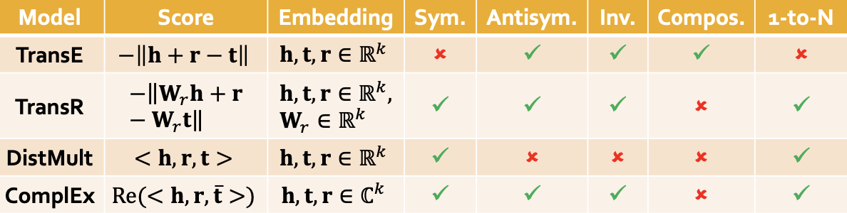
These methods can not model hierarchical relations
Difference: how they are thinking the geometry of the relation, and how to move around in the space
people don't combine shallow embedding with neural network
Lec11 Reasoning over KGs
- multi-hop query
- difficulty: the KG is incomplete and unknown, missing relations;
- completed KG is dense graph
- so implicitly impute and account for the incomplete KG
- Two ways:
- Embedding query into a single point (like TransE)
- Embed query into a hyper-rectangle(box)
- Two ways:
Predictive Query
- Types:
- one-hop-query:
- find the tail
- (e:Fulvestrant, (r:Causes))
- Path query: (e:Fulvestrant, (r:Causes, r:Assoc))

- Query plan of path queries is a chain
- Traverse the graph
- ouput: a set f nodes
- Conjunctive Query: ((e:BreastCancer, (r:TreatedBy)), (e:Migraine, (r:CausedBy))
- start from 2 entity
- KG Completion <-> One -hop query
- one-hop-query:
- Difficulty: KG is incomplete and unknow
- completed KG is a dense graph, time complex
- traversal problem -> prediction task
- Task: answer path-based queries over an incomplete knowledge graph
- generalization of the link prediction
- Hypergraph: a link connects a lots of nodes
Answering predictive queries
- Map graph & query into embeding space
- answer are node close to query
- Idea 1: Traversing KG in vecotr Space
- generalize TransE
(r: learned relationship embedding) - t: potential tail
- Multi-hop:
- TransE can not model 1-to-n relatiosn, so Query2box can not handle 1-to-N
- TransE can handle composititonal relations
- Can we answer logic conjuction operation
- set intersection

- gray node in the picture is a set of entities
- Idea2: Query2Box
Query2Box
query -> box
- intersection of 2 boxes is a box
- Things to learn:
- entity embedding : zero dim box
- Relation embeddings: 1 dim box
- intersection operator f
- optimize the node postiion and the box and operator together, so the nodes in the box
- Things to learn:
- for every relation embedding r -> projection Operator P
- cen
- off
- Box: a set of nodes

- move and resize the box using
- Geometric Intersection Operator 𝓘 -> learned
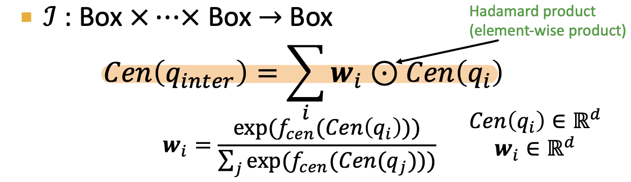
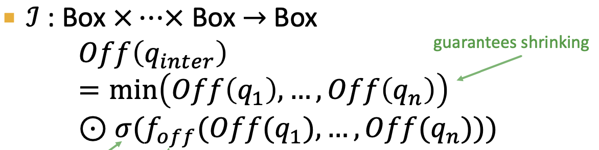
to extract the representation of input box
- score function:
- L1 distance
- if the entity is inside box:
- if outside, need to add
- d_box(q, v):

- f= -d_box
- outside box: a lot of penalties; inside box, a little bit penalty
- intersection could happen at anywhere in the query(could at early stage)
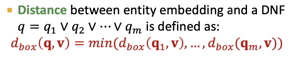
- How to implement AND-OR query?
- Union is impossible -> Allowing union over arbitrary queries requires high-dimensional embeddings

- For 3 points, 2-dimension is OK. 4 point is not OK.
- If we want to "v2 or v4", but do not want v3, we cannot do that in 2-dimensional. We need another dimension to take v3 out.
- take all unions out and only dounion at the last step
- Union at last step
- Disjunctio(分离) of conjunctive queries
- Union at last step
How to Train
- Trainable parameters:
- Relation: 2 vectors:
- one to move the box into embedding space
- one to resize
- Entity embeddings
- Intersection operator
- Relation: 2 vectors:
- traing set = query + anwsers + negtive anwsers (non - anwser)
- maximize the score 𝑓" 𝑣 for answers 𝑣 ∈ 𝑞 and minimize the score 𝑓"(𝑣′)

- start with the anwser entity and go backwards
- wheter we can try to excute the query plan backward
- Steps of instantiated query q?
- start with query template (viewed as an abstraction of the query)
- generate a query by instatiating every variable with a concrete entity and relation from the KG
- Start from instatntiating the answer node; randomly pick on entity from KG as the root node,
- Ranomly sample one relation asscicated with current entity
Example
string insturment ---(projection)---->a set of different string instruments --(projection)---> the instrumentalists who play string instruments
FP/false positive: not play string instruments but in the box
- FN: who play string instruments but not in the box
Lec12 Motif
Fast Neural Subgraph Matching and Counting
Subgraphs and Motifs
- node-induced subgraph
- edge-induced subgraph
- Graph isomorphism:
- G1 map to. G2, bijection
- Subgraph isomorphism
- Graph-level frequency:
- hom much subgraphs induced by differetn
- hom much subgraphs induced by differetn
- Node-level subgraph frequency definition
- Node-anchored subgraph
- motifs:
- Pattern
- Recurring: frequency
- Significant: random
- Graphlet is used to define what happens with a given node
- graphite has a root,
- Motif do not have a center
- Subgraph frequency
- number of unique subsets
- Node-level Subgraph Frequency:
- Anchor map to different nodes
- Motif Significance
- Subgraphs that occur in a real network much more often than in a random network
- Generating random graph - NULL model
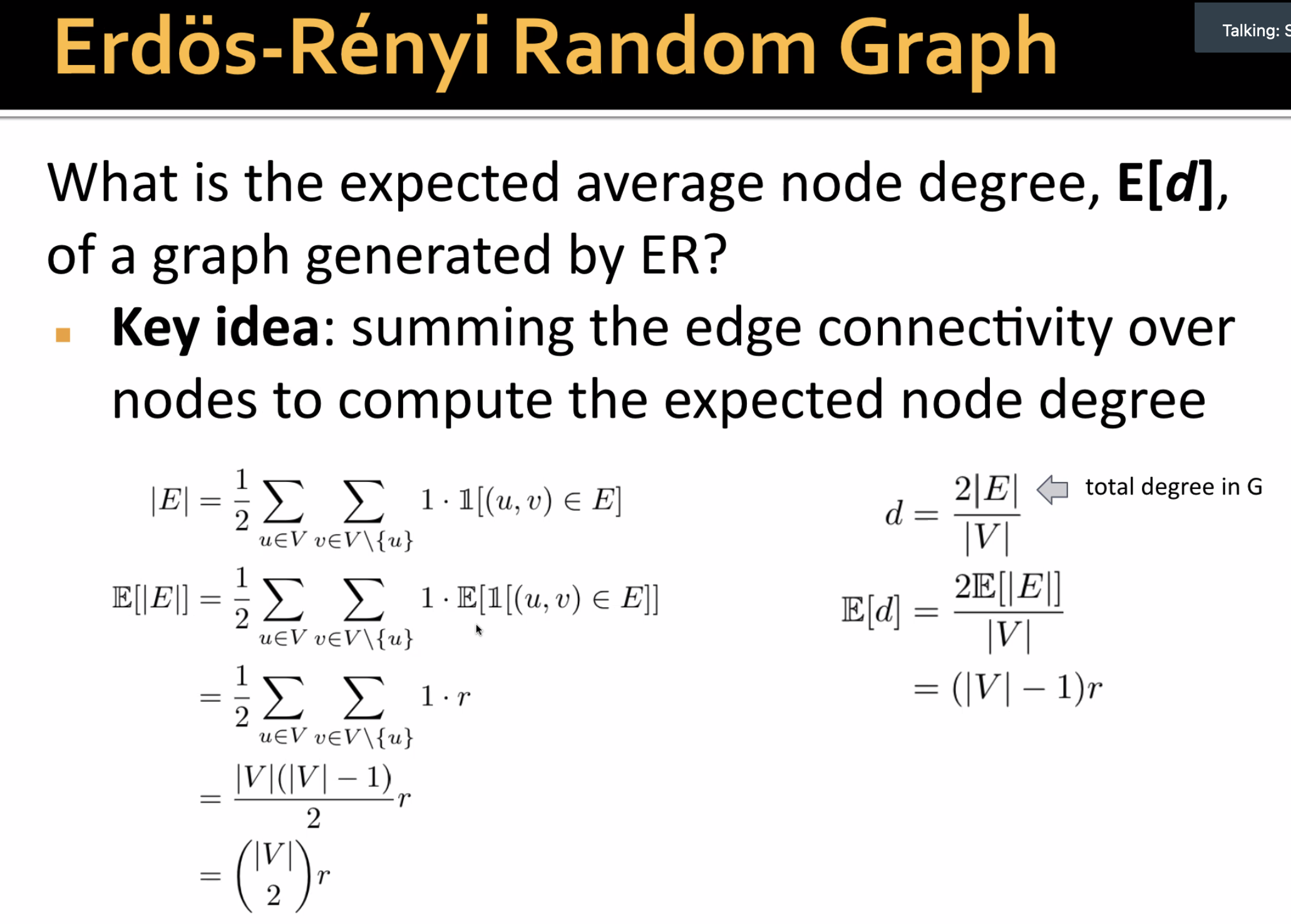
- ER random graph
- create n ndoes, for each pair of nodes (
) flip a biased coin with bias 𝑝
- create n ndoes, for each pair of nodes (
- Keep same degree of the nodes, generate random graph
- create nodes with spokes
- randomly pair up mini-nodes
- Generate random graph: switching
- select a pair of edges and exchange endpoint
- nodes keep it's degree
- computationally complex
- ER random graph
- Use statistical measures to evaluate how significant is each motif
- use Z-score
- negtive value: under-representation
- positive value: over-representation

- Network significance profile(SP): normalized Z-scores
- use Z-score
Subgraph Representations/Matching
Task: is a query graph a subgraph in the target graph
Do it in embedding space
- consider a binary prediction
- work with node-anchored definitions
decompose input big graph into small neighborhoods
Steps:
- using node-anchored definitions, with anchor
- obtain k-hop neighborhood aroud the anchor
embedding
is less than or equal to in all coordinates - Order Embedding Space partial ordering
- non-negtive in all dimensions
Subgraph isomorphism relationship can be encoded in order embeeding space
- Transitivity:
- Anti-symmetry
- Closure under intersection
Loss function: max-margin loss

Train on positive and negitve examples
- learn from postivie and negtive sample
- positive sample: minimize loss function
- negtive sample: minimize max(0,
-E(Gq,Gt)) - prevents the model from learning the degenerate strategy of moving embeddings further and further apart forever
Generate positive and negative examples
- use BFS sampling
Subgraph Predictions on New Graphs
- Gq: query, Gt: target
- reqeat check for all
Traverse every possible anchor
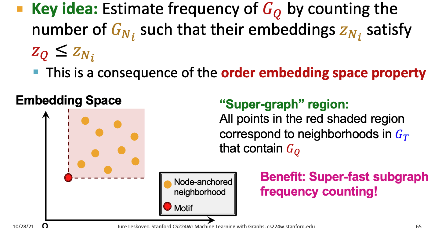
Finding Frequent Subgraphs
Representation learning
SPMiner: identify frequent motifs
- Decompose input graph
into neighborhoods - Embed neighborhoods into an order embedding space
- Grow a motif (Motif walk) by iteratively chossing a neighbor in
- Decompose input graph
Super-graph region:
Motif walk
Lec13 Recommender System
Recommand System as bipartite graph
- Given: past use-item interaction
- Task: preidct new items each user will interact in the future
- link prediction task
- recommend K items
- K is very small
- Evaluation Metric: Recall@K
Embedding based model
- training recall@K is not differentiable
- Two surrogate loss function (differentiable)
- binary loss
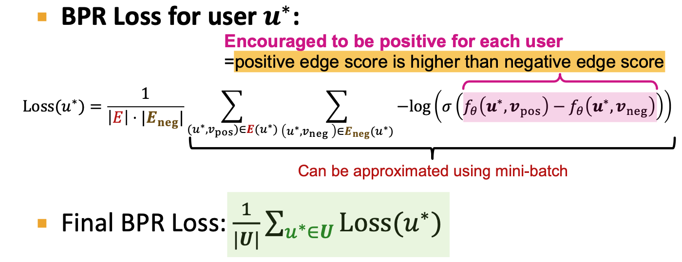
- Bayesian Personalized Ranking loss:
- Positive edges and negtive edges
- Binary loss pushes the scores of positive edges higher than those of negative edges
- Binary Loss Issue:
- only consider all the positive edges
- not consider personallize, not consider every user.
- Metric is personlized.
- BPR(Bayesian Personalized Ranking loss)
- define the rooted positive/negtive edges
- For a fix user, positive interaction score is higher than negtive users
- Average over users
- Collaborative filtering - Why embedding models work
- useing collaborators to filter the items
- Embedding-based models can capture similarity of users.
Nerual Graph Collaboratvie Filtering
no user/item features
based on shallow encoders

- only implicitly captured in training objective
- if u, v has an edge, the f should be high
- Only the first-order graph structure
NGCF
- explicitly incorporates high-order graph structure when generating user/item embeddings
- ordiniral GNN has user/item features, learn GNN parameters
- no node feature, so can not directly use GNN
- NGCF jointly learns both user/item embeddings and GNN parameters
- Steps:
- prepare shallow embedding
- use GNN to propgate the shallow embeddings
- different GNN parameters for user and for items
LightGCN
- NGCF learns two kinds of parameters
- shallow learnable embeddings are quite expressive
- Overview of LightGCN:
- Adjacency matrix
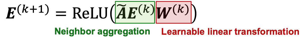
- Use matrix formulation of GCN
- Simplification of GCN - removing non-linearity
- Simplifiying GCN
- Diffusing node embeddings
- GCN:
- Diffusion Matrix
- Diffusion Matrix
- Simplifiying GCN:
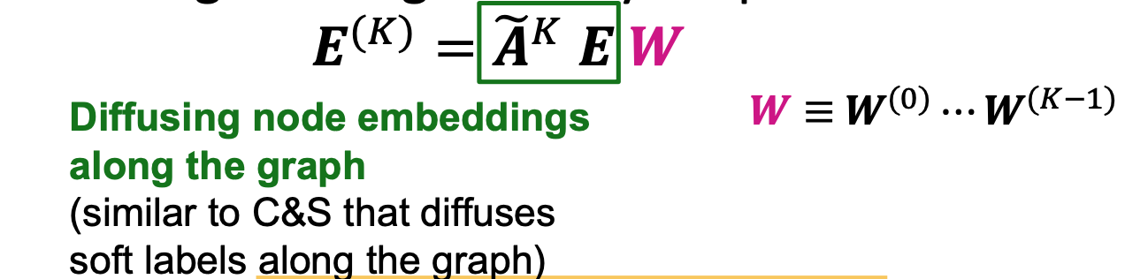
- remove ReLU

- each matrix multiplication diffuses current embeddings to their one-hop neighbors
- Multi-Scale Diffusion
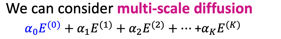
- hyper-parameters
- take the embeddings of every layer and average (LightGCN)
- Similar uses share common neighbors and are expected to have similar future preferences
- not able to deal with new products - all the items should be available when training
- cold start problem of the recommend system
- Difference from GCN:
- GCN add self-loop in neighborhood definition
- LightGCN: self loop is not added in the neighborhood definition
- Difference from MF:
- MF uses shallow user/item embeddings for scoring
- LightGCN uses diffused user/item embeddings for scoring
- LightGCN: learnable parameters are all in the shallow input node embeddings (E)
PinSAGE
- not learning shallow embeddings for user/items.
- if learn, it's not inductive; PinSAGE is inductive
- picture 2 picture recommend
- pictures pin to same board
- key idea:
- share the same set of negtive samples across all users in a mini-batch
- Curriculum learning:
- hard negative example: thank you card and happy brithday card
- make extremely fine-grained predctions / add hard negtive
- at n-th epoth, add n-1 hard negative items
- generate hard negtives: take item from another recommend system 200th - 5000th;
- itemn ode that are close but not connected to the user node
- hard negtive are shared within mini-batch
- Negitve sampling: sample from different distance
Lec14 Community Detection
Flow of Information
Two persepective on friendships:
- link from a triangle: strong link
- long-range edges allow you to gather information from different parts of the network and get a job
- Weak link: long-range edges
- Strong relationship within clusters, weak relationships connect different clusters
- clusters: friend's friend is easy to become friends;
- link from a triangle: strong link
Triadic closure = high clustering coeffcient
Edge overlap:

Network Communities
- How to discover clusters
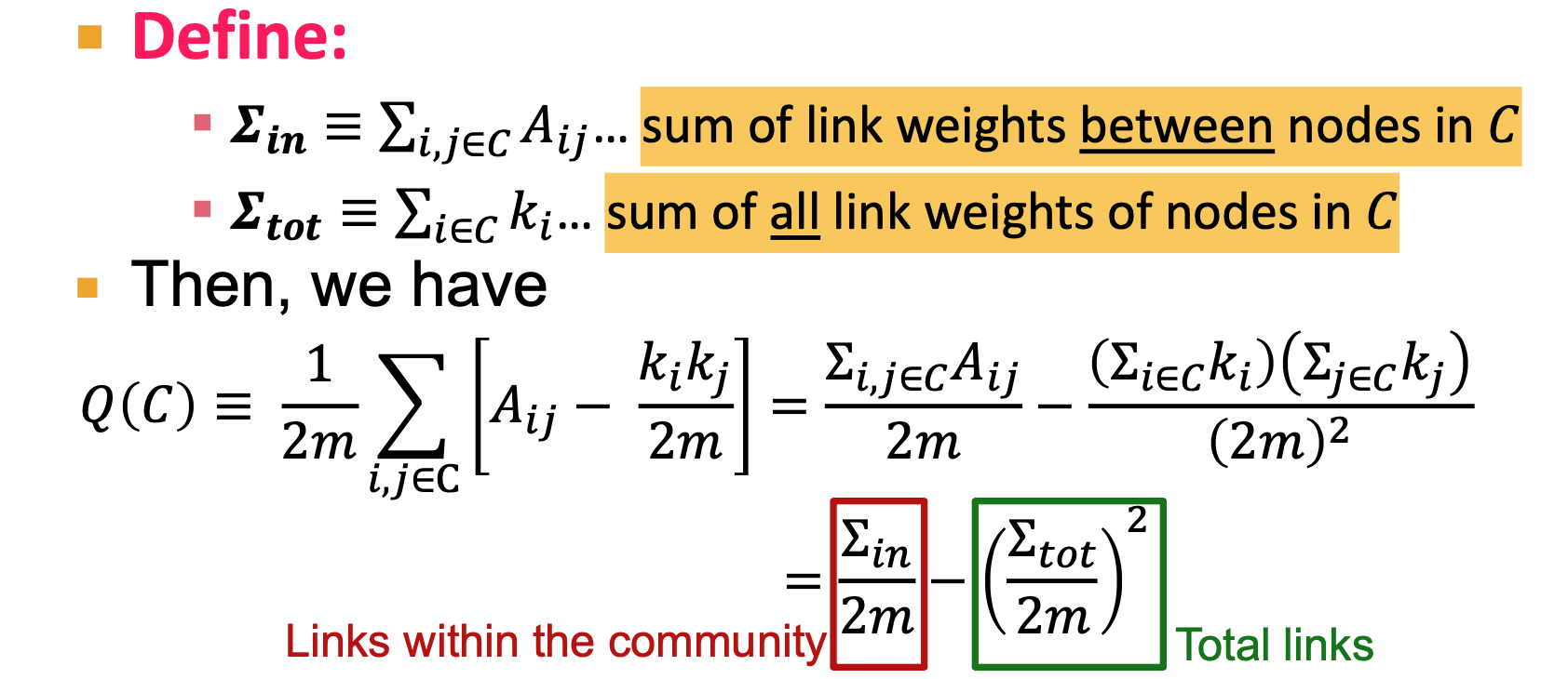
- Modularity Q: measure of how well a network is partitioned into communities
- Need a null model
- Null model: Configuration Model
- same degree distribution, uniformly random connections
- 2m: total 2m half-edges
- multigraph
, for every edge of i, times the probability of have an edge wih node j 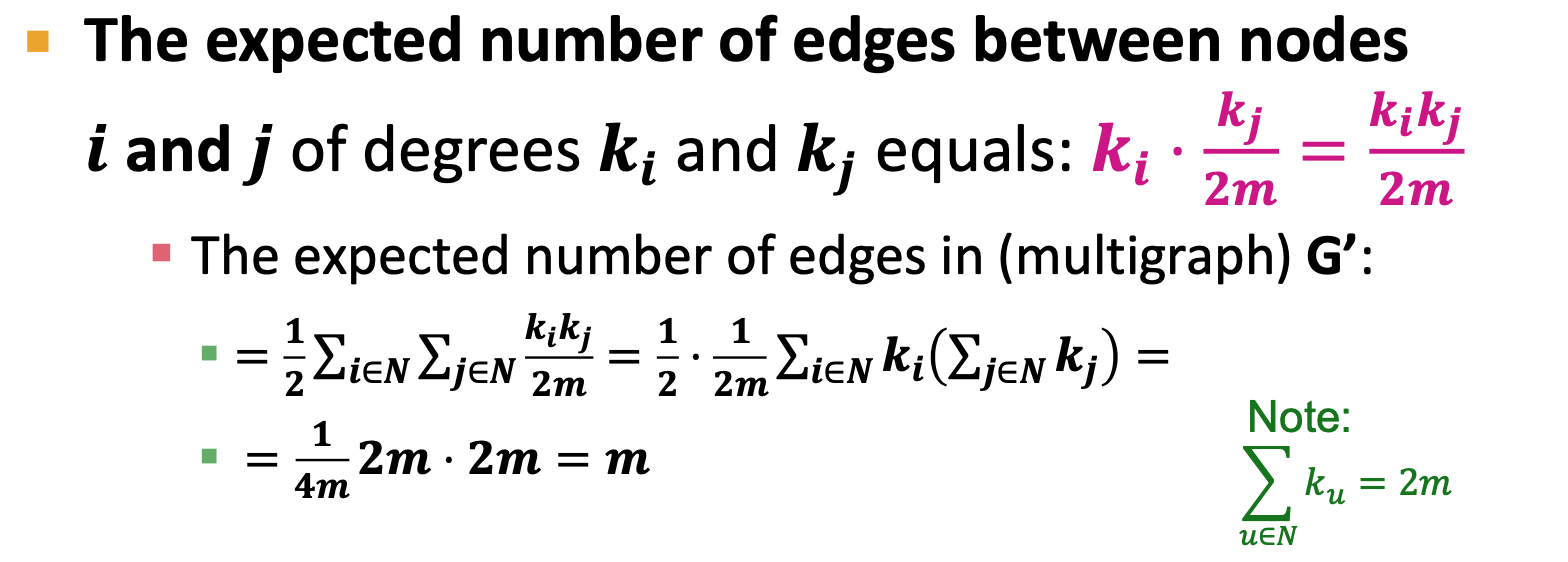
- Modularity Q=0, no cluster structure
- Modularity applies to weighted and unweighted networks
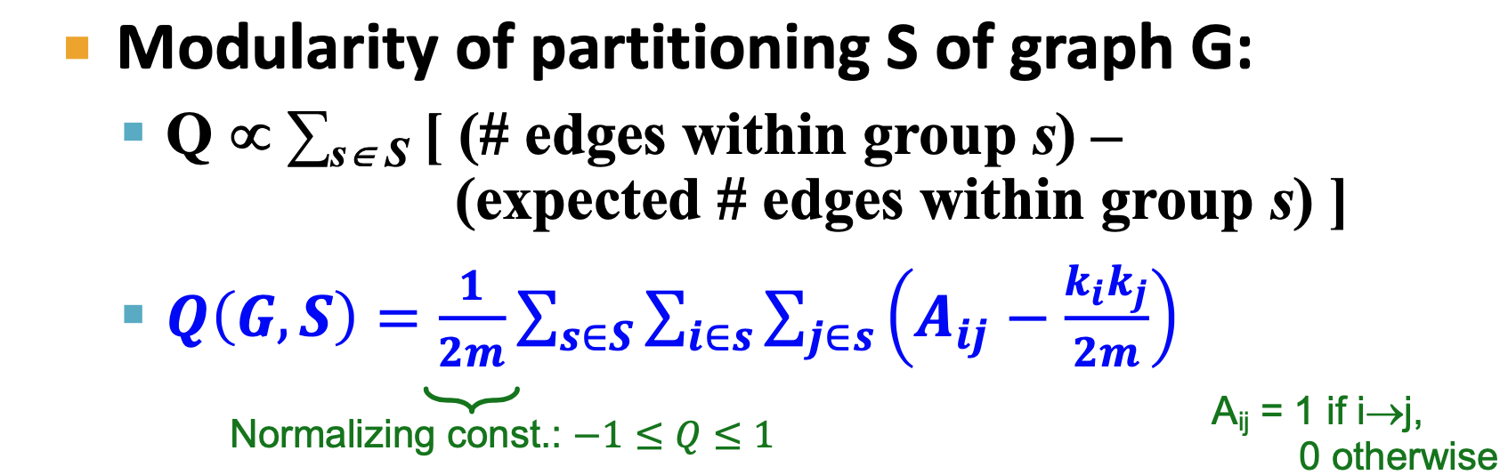
- k_i, k_j are degree of the node
- Q= -1, anti-community. We call us a community, but common friends are in another group
- Q=1, well structured community
- Modularity applies to weighted and unweighted networks
- We can identitfy communities by maximizing modularity
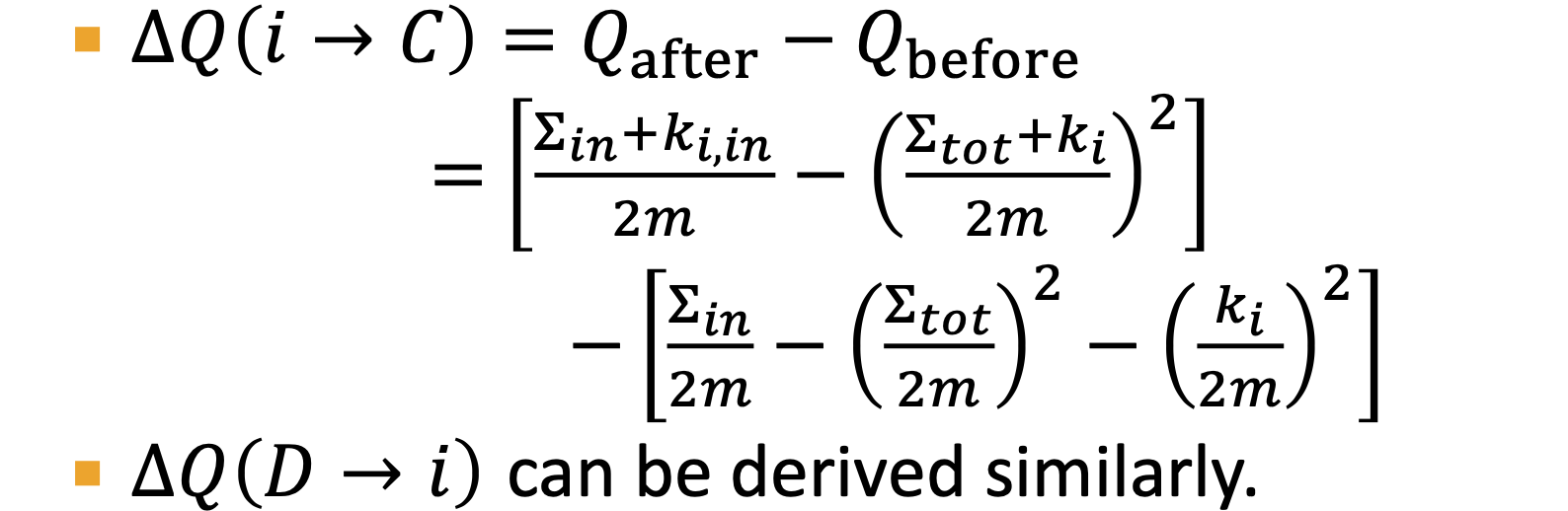
Louvain Algorithm: community detection
- greedy algorithem
- Phase1: Modularity is optimized by allowing only local changes to node-communities memberships
- Phase2: group into super-nodes, consider as a weighted graph
- weight = number of edges in the original graph
- hierachical structure, 启发性的
- Output of Louvain algorithm depends on the order the nodes are considered
- Calculating
- Within community: counting 2 times every edge
- edge between community: counting 1 time (actually twice, half into one end, another into another end)
- Can NOT decided the number of communities ahead

Detecet overlapping Communities
the model is a bipartite graph
- community nodes
- Original nodes
- relationship: menberships M
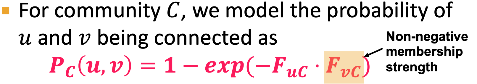
AGM: generative model:
- generate from bipartite graph to a network
Target: from an unlabeled graph, generate bipartite graph
- Given F, generate a probability Adjanct matrix
- Maximum likelihood estimation
- Given real graph G and parameter F
- relax AGM:
- node u and v can connected via mltiple communities
size: # community * # number of nodes - Log likehood: avoid super small value
NOCD model:

- Use log-likelihood in target function:
- Neural Overlapping Community Detection(NOCD)
- use GNN to learn F, learn
and - Real-world graphs are often extremely sparse.
- model spend a lot of time on edges don't exsit
- Use negtive sampling to approximate the second item(edges not exist )
- inside a given batch
- Decide the number of communities:
- look at objective function, change number of communities and see the change of L(F)
Lec15 Deep Generative Models for Graphs
Graph generation
Graph Generation: Deep Graph Decoders
- only have access of samples from p_data
- learn p_model, then sample more graph from p_model
- Goal:
- graph model fitting: get
- maximum likelihood
- generate more sampling
- graph model fitting: get
- Auto-regressive models:
- chain rule:
- based on previous steps/ generate results
- chain rule:
GraphRNN:
RNN:
hidden state + input => output
RNN for sequence generation. deterministic
generate graph sequentially: sequentially adding nodes and edges
A graph + a node ordering = A sequence of sequences
- learn to how to print adjacency matrix
- add node x, ask node x who connect to him
Node-level RNN & edge level RNN
We want our model stochastic, not deterministic
- flip a coin with bias
to decided whether the edge exist. - output
is a probability of a edge existence
- flip a coin with bias
Training:
- RNN get supervision every time
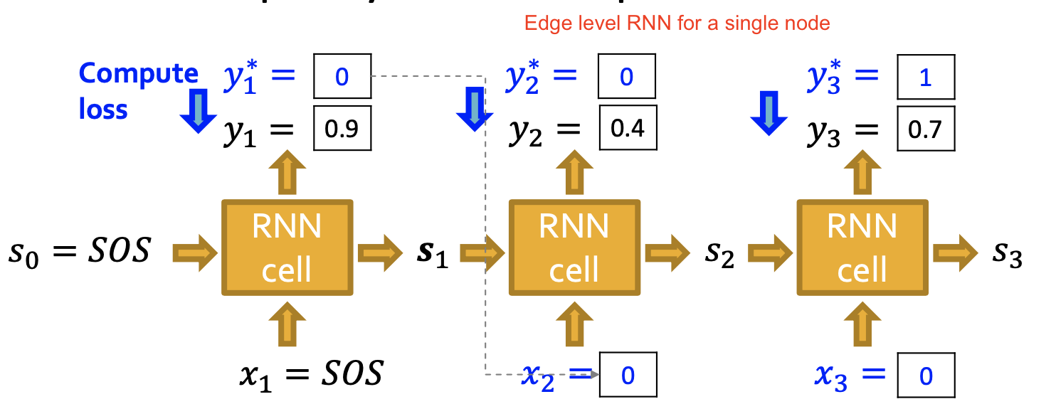
- Edge level RNN only predict the new node will connect to each of the previous node
- RNN get supervision every time
Test:
- use GraphRNN's own predictions
Node ordering - BFS
- Benefits: 1. reduce possible node orderings; 2. reduce steps for edge generation
How to compare two graph statistics: Earth Mover Distance (EMD)
How to compare two sets of graph statistics
- Maximum Mean Discrepancy (MMD) based on EMD
GCPN: combines graph representation + RL
- GNN captures graph hiddent state explicit
Exam Prep OH
- Miscellaneous Problems