CS231A Lecture Notes
Lec2 Camera Model
Pinhole cameras & lenses
Pinhole Camera:
Aperture is too large: blur picture
Aperture too small: not enough lights
Cameras & lens
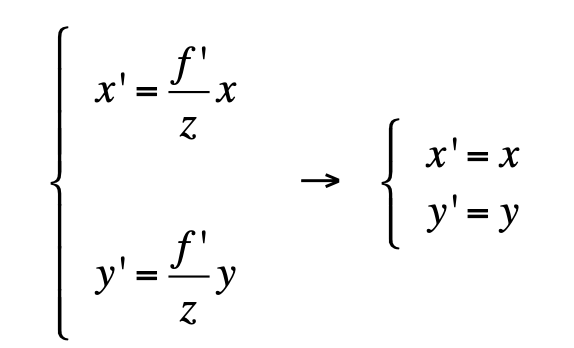
a sepcific distance to ???
all rays of light that are emitted by some point P are refracted by the lens such that they converge to a single point P ′
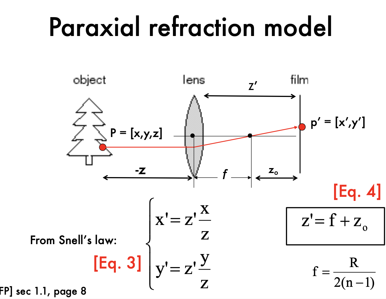
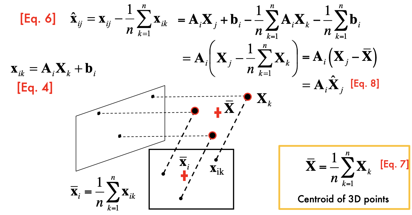
- all the x, x' are in camera reference system
Radial Distortion:
- noticebale for rays that apss throught the edge of the lens
Is the projective transformation correspond to what we see in actural digital images: No
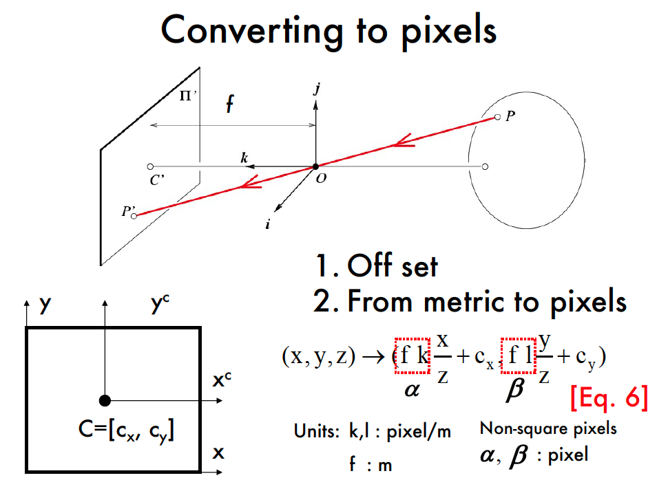
points in the digital images are, in general, in a different reference system than those in the image plane.
digital images are divided into discrete pixels
the physical sensors can introduce non-linearity such as
distortion to the mapping.
Euclidian:
- projective transformation is non-linear in Euclidian Space
- can not express in matrix form
Homogeneous coordinate system
- add one dimension at the last dimension
- projective transformation is linear
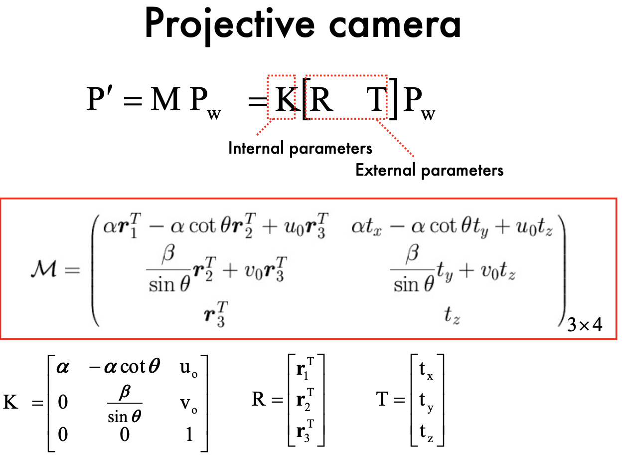
- Projective transformation - Intrinsic matrix
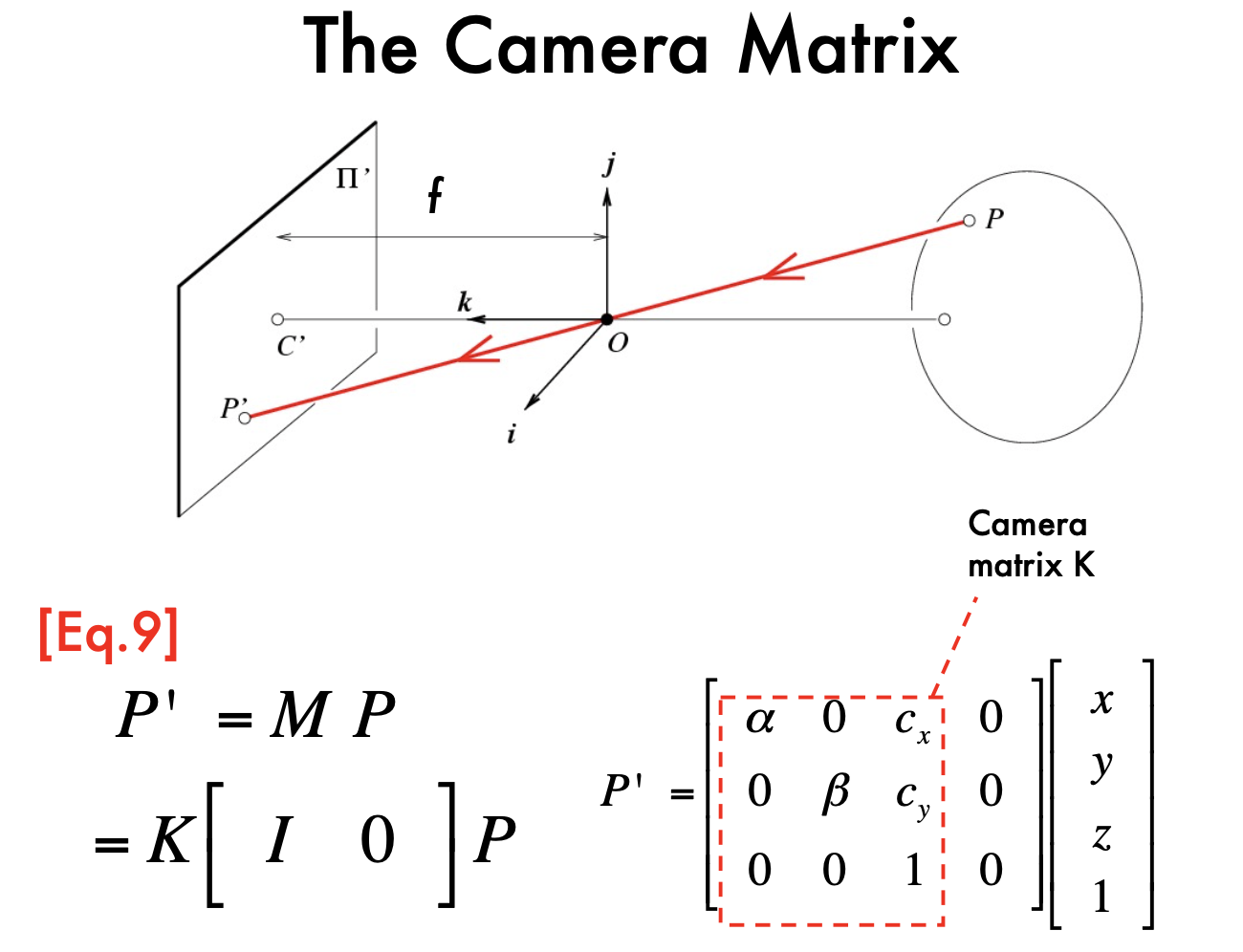
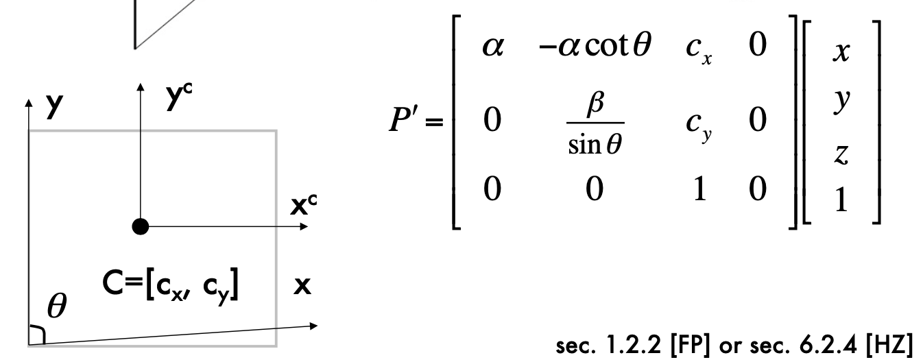
- Add camera Skewness: 5DoF
The geometry of pinhole camera
World reference system (Appendix A) - Extrin
Translation in Homogeneous Coordinate: (2D)
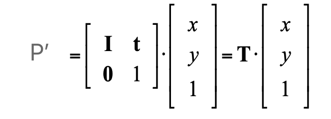
R: rotation
- Euclidean:
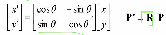

- Euclidean:
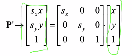
S: scaling in Homogenous Coordinate (2D), 1 DOF
- 3D rotation: 3 DOF. dimension: 3 (for 3D point; For 2d point, the dimension of R is 1) We can rotate around x, y, z axes
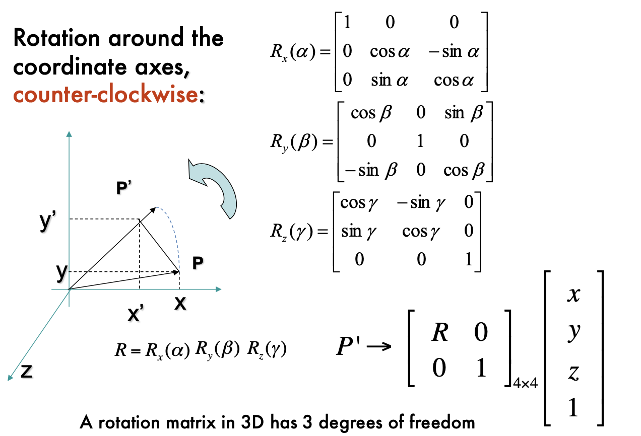
- 3D rotation: 3 DOF. dimension: 3 (for 3D point; For 2d point, the dimension of R is 1) We can rotate around x, y, z axes
World reference system => Camera reference system
- R: totation
- T: translation

R, T extrinsic parameteres, only related to exteranl coordinate system
- K, intrinsic parameter: only about the camera system
- 5 dimensions of K: alpha, beta, Cx, Cy, theta
- K, intrinsic parameter: only about the camera system
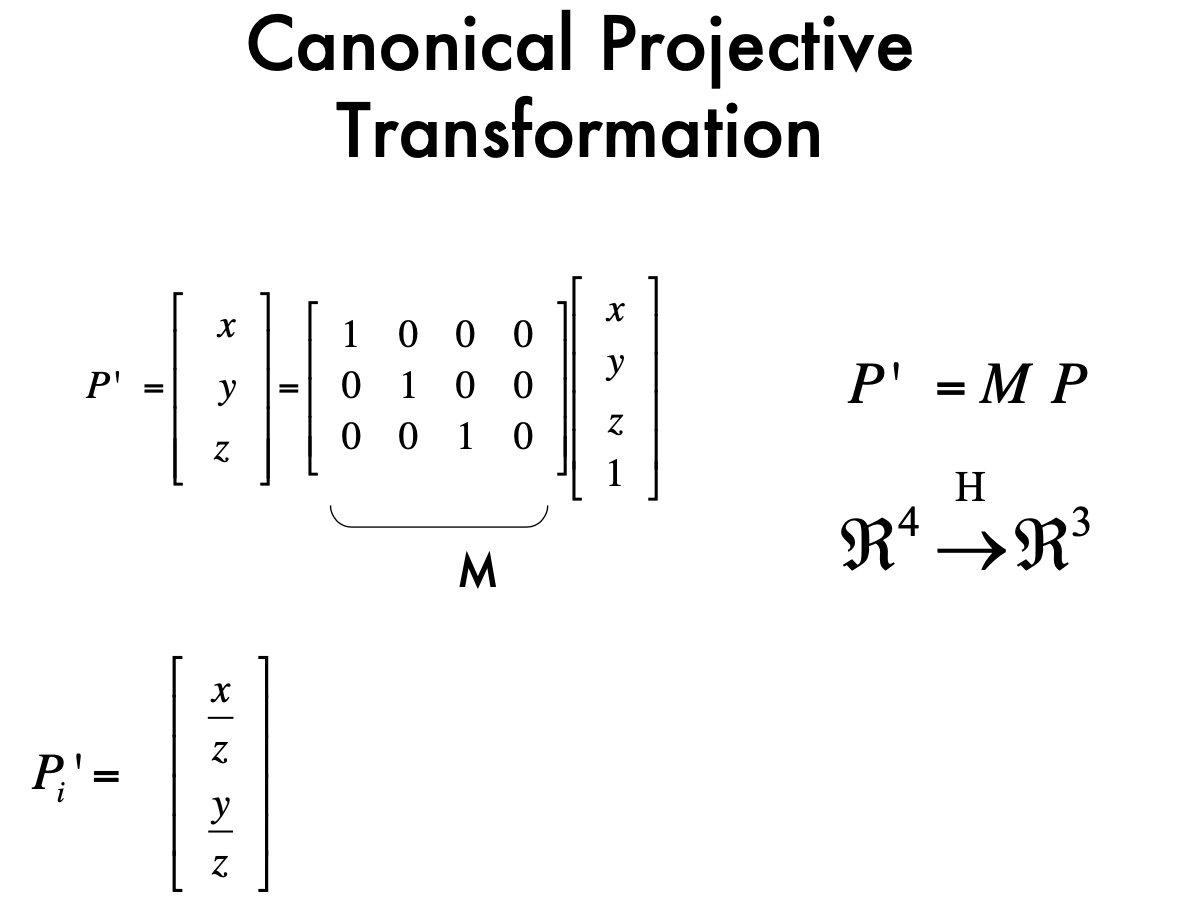
Projective transformation:
- M's dimension: 11
- K =5, R=3, T=3 , total 11
- M's dimension: 11
Projection properties
- point to point
- lines to lines
- for fish cameras, it's not true. line to skews
- distant objects look smaller
- length diviede by z (z is the depth/distance)
- parallel lines intersect in the image at vanising point
- Horizon line (vanishing line) is always a straight line
Canonical Projective transformation
Lec3 Camare Model2 & Camera Calibration
- Recap:
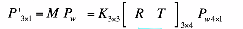
- Exercise: In homogeneous system: If the coordinate of world system and camera system is the same: [R T] = [I 0]
- Assume caemra model as a focal length, zero skewness, no offset, and pixel are squrae:
 (no skew, no offset,)
- K, camera matrix:
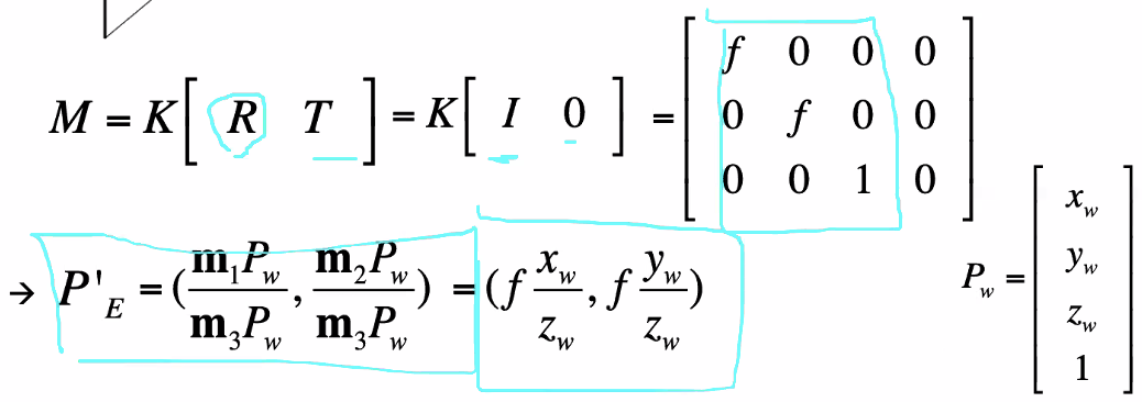
- Weak perspective projection
- remove non-linearity
- When the relative scene depth is small conpared to its distance z_o form the camera
- reference plane: can be assigned to any
- in Euclidan, the
simplified 
- Orthographic projection:
- the optical center is located at infinity
- Pros and cons:
- weak perspective is much simpler, useful for recongnition
- Pinhole perspective is acurate, useful for SLAM
Camera Calibration
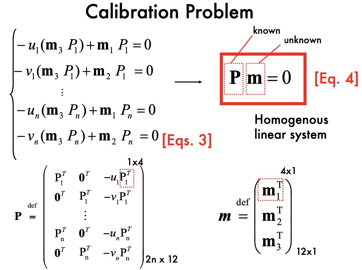
Calibration:
- Estimate intrinsic and extrinsic parameteres from 1 or multiple images
- Calibration rig: a typical rig is a cube. The corner is the original point of world reference system
- 11 unknow parameters, at least 6 corresponding point pairs (each point has 2 equations)
- P is homogenous coordinates
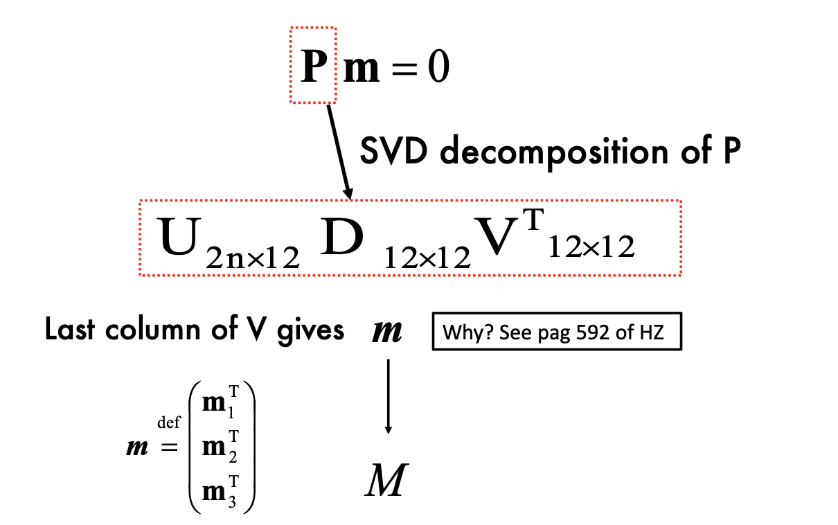
- Solve by SVD:
- Degenerate case: all the point pairs should NOT belongs to a line or even a plane;
- Points cannot lie on the intersection curve of two quadric surfaces
- Use
to correct scale issue (the matrix is up to scale)
Handling distortions
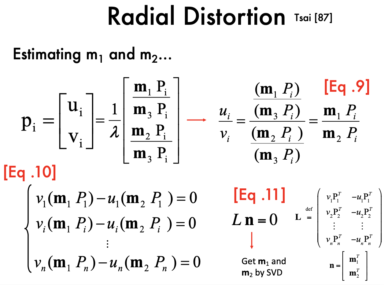
start by solving linear problem (
) Another method: estimate m1 and m2 and ignore
- the slope is constant: u_i / v_i
- first solve m1 and m2, then compute m3
Radial Distortion:
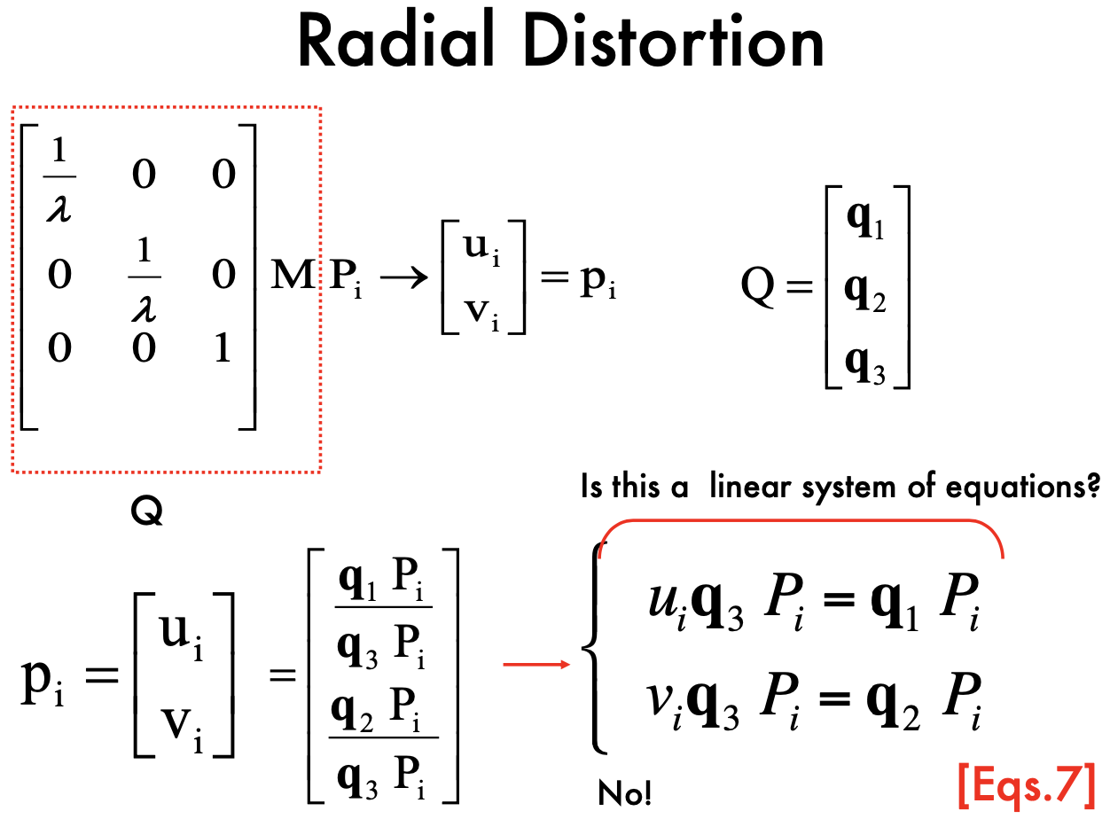
- Not a linear system
Solve: use slope

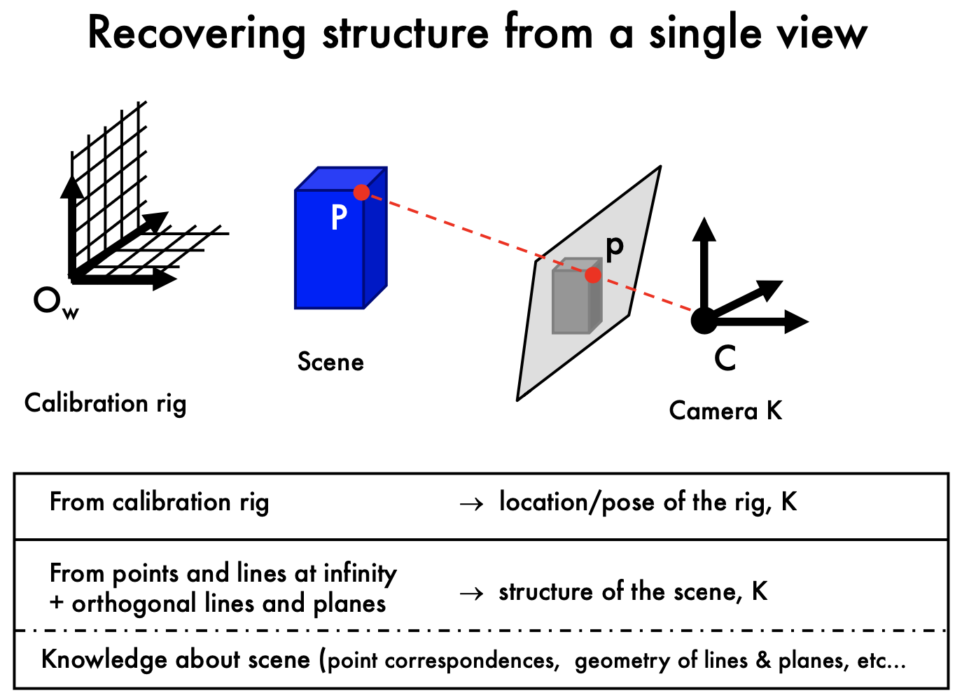
Lec4 Single View Metrology
Can I estimate P form the measurement p from a single image?
- We only know P is on the red line, but we do not know where P is.
- Can not map from 2D to 3D
Transformation in 2D
- Isometry: concate of rotation and translation
- disscuse in homogenous space
- preserve distance (areas)
- Rotation + Transformation
- DOF =3, degree of freedom (rotation:1, translation: 2)
- Similarity:
- Unifom Scale, Rotation, translation
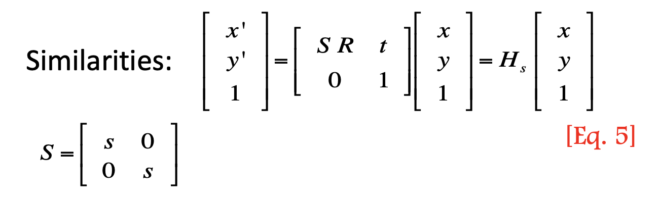
- DOF = 4 (rotation:1, translation: 2, scale:1)
- preserve the ratio of length
- Unifom Scale, Rotation, translation
- Affine:

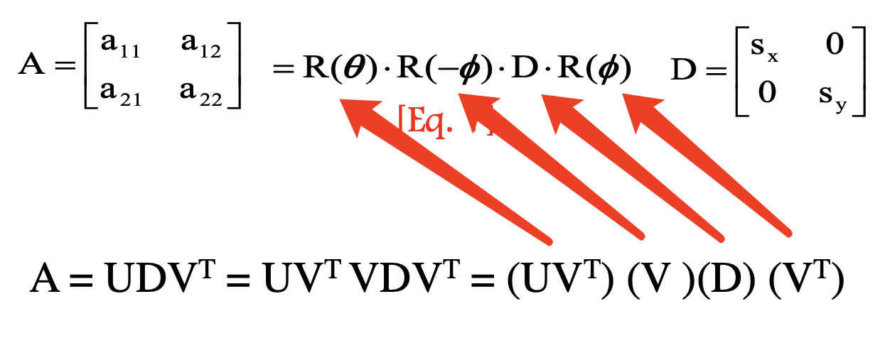
- First rotate
, then scale, then rotate back ,then rotate - D: anisotropic scaling
- Preserve parallel lines,
- DOF: 6 (4 from matrix A, 2 from D)
- Projective transformation:

- 8 DOF ???
- Isometry: concate of rotation and translation
Vanishing points and lines
l: [a b c] (in 2D)
x belongs to l,
intersecting lines:
Points at infinity: [x1, x2, 0]
lines in 2D plane
- lines infinity: [0 0 1]
- Points and lines at infinity:
- Projective transformation of a point at infinity
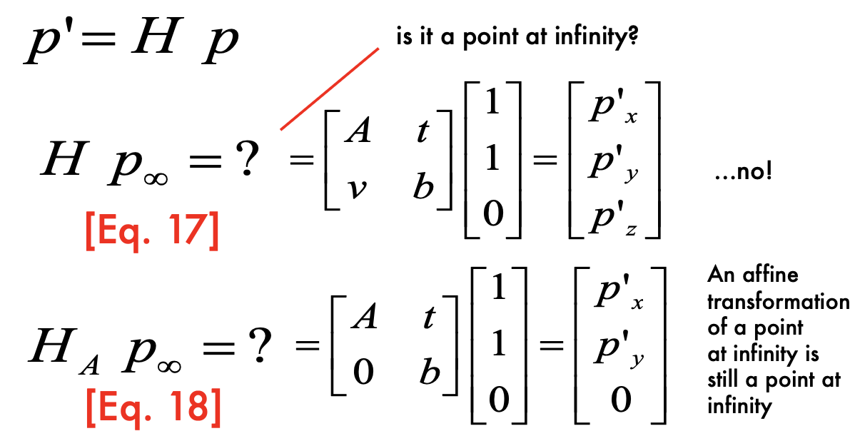
- apply H for p_infinity:
- is it a point at infinity? No
- A is 2*2, v is a vector (1* 2 vector) to capture project ???, b does not matter
- when v=0, it is a point at infinity [Px, Py, 0]
- Apply affine transformation: still a point at infinity
- Projective transformation of a point at infinity
- Projective transforamtion of a line:
- when H= HA, its a line at infinity
planes and points in 3D:
,
lines in 3D:
- Vanishing points
 yes
yes- M = K [R t] maps point in 3D into image, p = Mx
- vanishing point is not at infinity
- v = Kd
- K, camera matrix; d, diretion of the line in 3D respect to camera
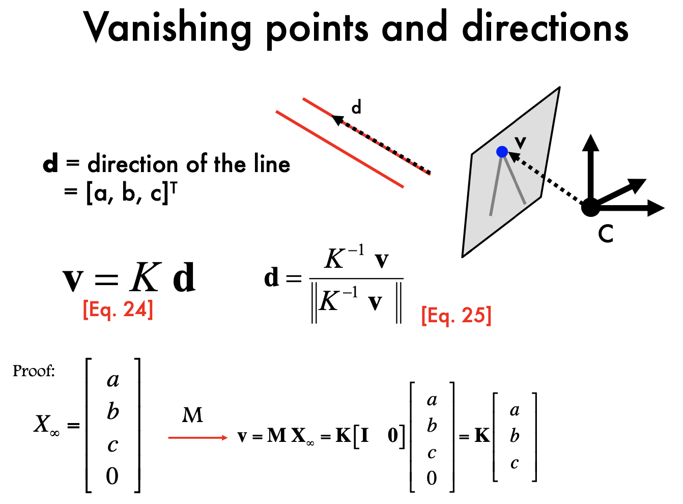
- Vanishing points
horizontal lines:
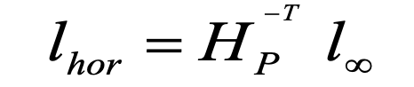
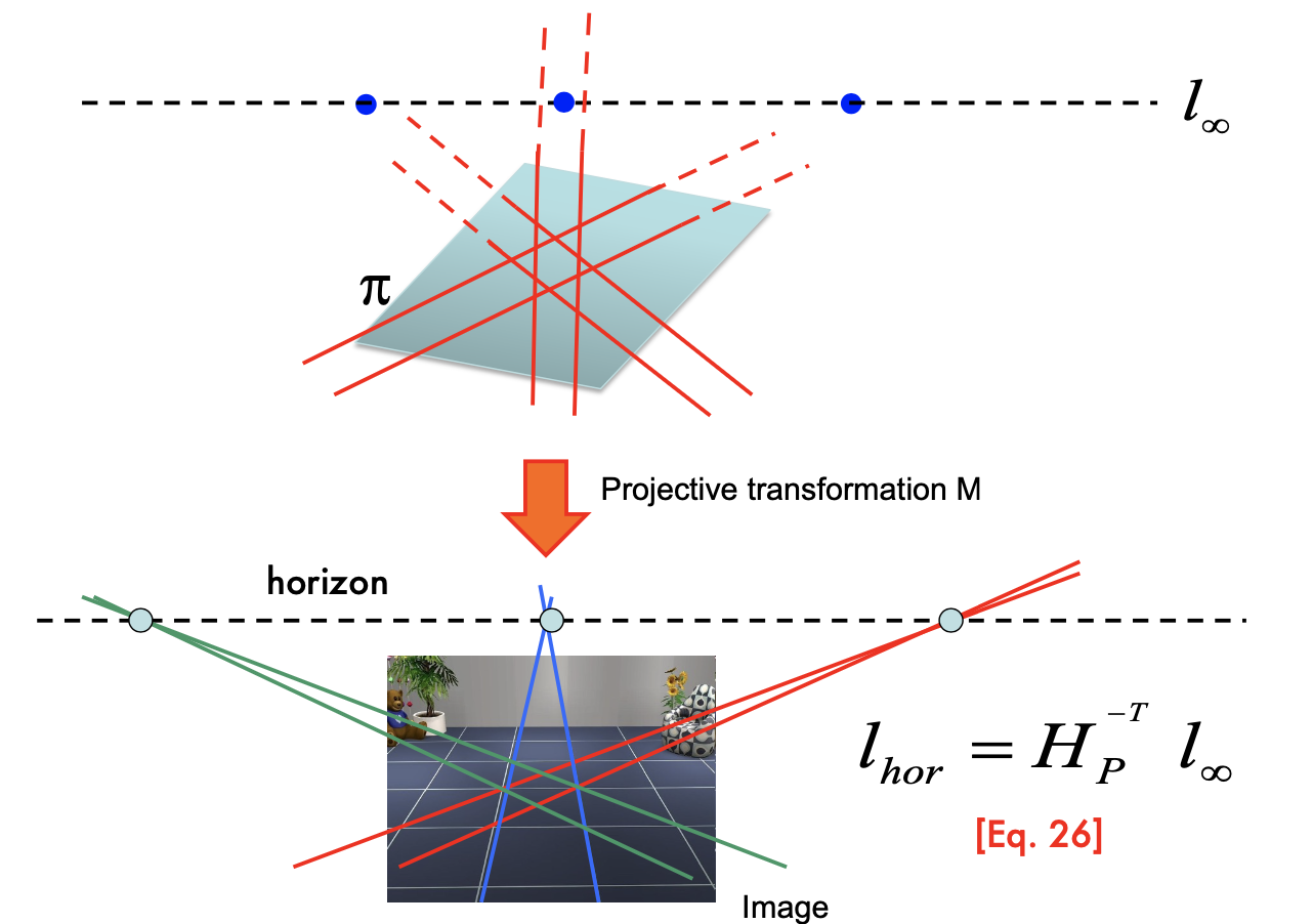
- Are these two lines parallel?
- Recognize the horizon line Measure if the 2 lines meet at the horizon if yes, these 2 lines are // in 3D
- Need to know the intersect point belong to horizontal
- originate at the same vanishing point -> parallel
Vanishing points and planes:
- n, the normal of plane
, calculate the normal in camera system 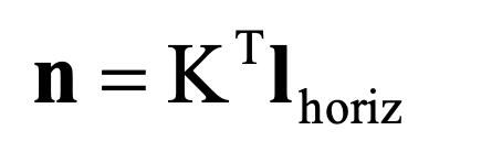
- A set of 2 or more lines at infinity defines the plane at infinity
- n, the normal of plane
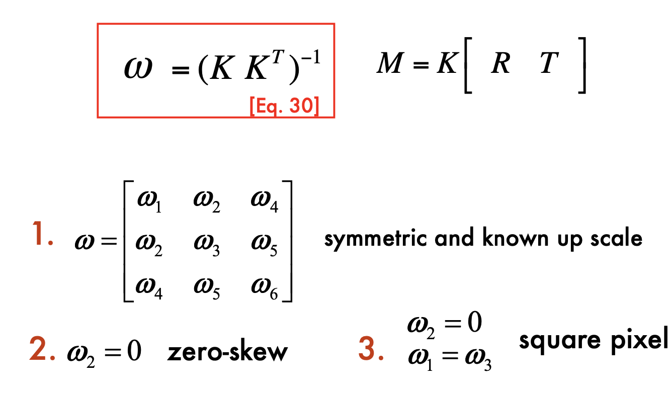
Angle between 2 vanishing points
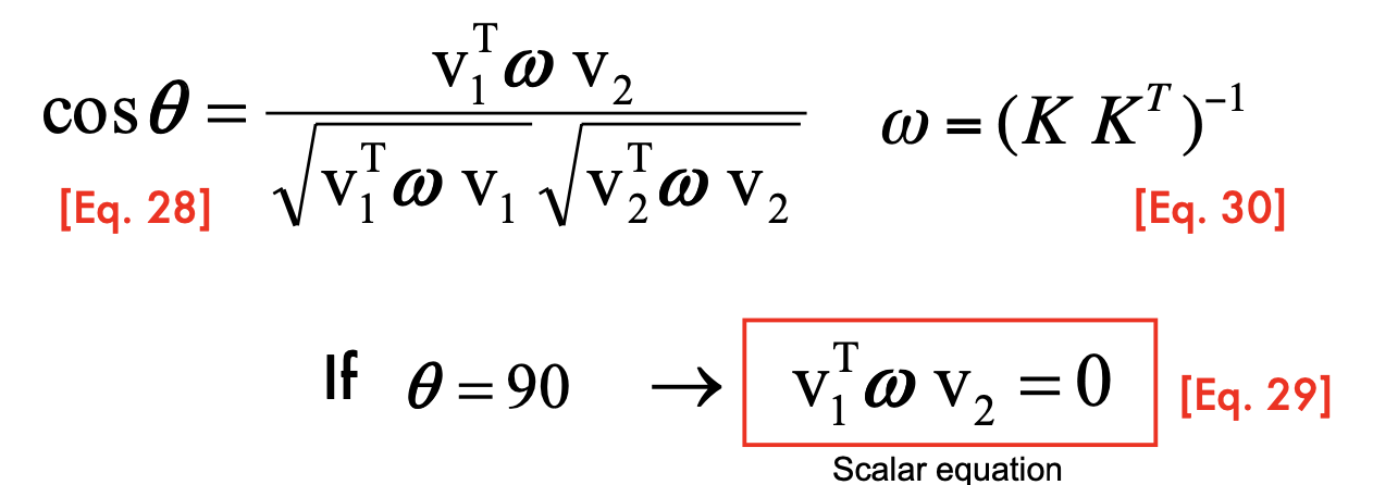
- Calculate K:
- useful to calibrate the camera; estimate the geometry of the 3D world.
Estimating geometry from a single image
A Single View Metrology Example
- we can measure v1, v2, v3 in image
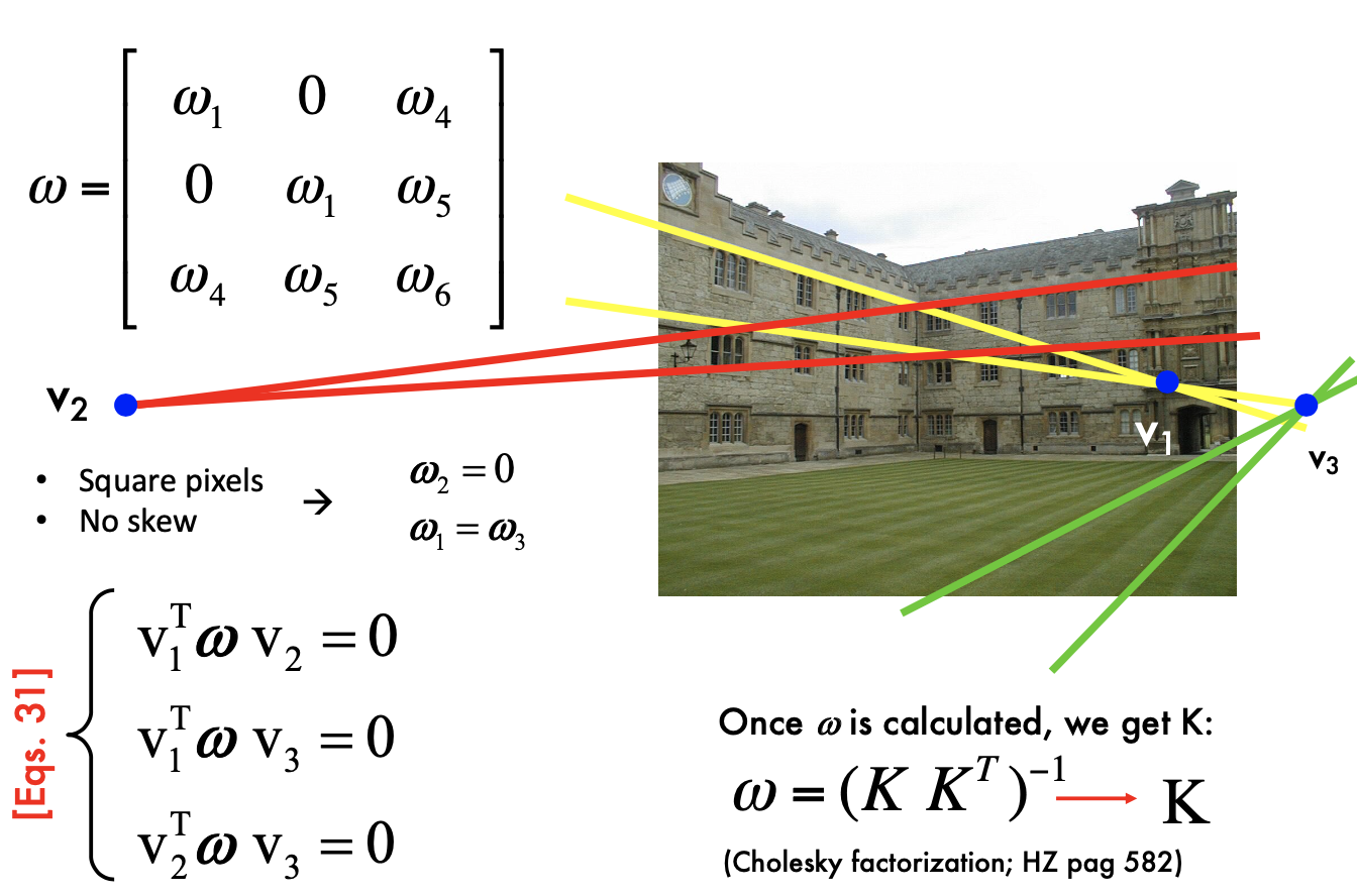
- using Cholesky factorization to solve K
- The equations are not sufficient for K, since K has 5 DOF
- the angle of each pair of plains is 90 (knowledge). If we do not have the knowledge, we can have ML methods
- with simplified camera model, we can calculate
using 3 points - normal n is in the camera coordinate system
- calculate normal n => reconstruction from single view
- the actual scale of the scene is NOT recovered
- we can measure v1, v2, v3 in image
Lec5 Epipolar Geometry
Epipolar Genometry = multi-view geometry
- Intrinsic ambiguity of the mapping from 3D to image (2D)
Two eyes help - Triangulation
- cross product of two line => intersection point, in homogenous system
- If there are some noise, the lines won't intersect
- find minimizes:
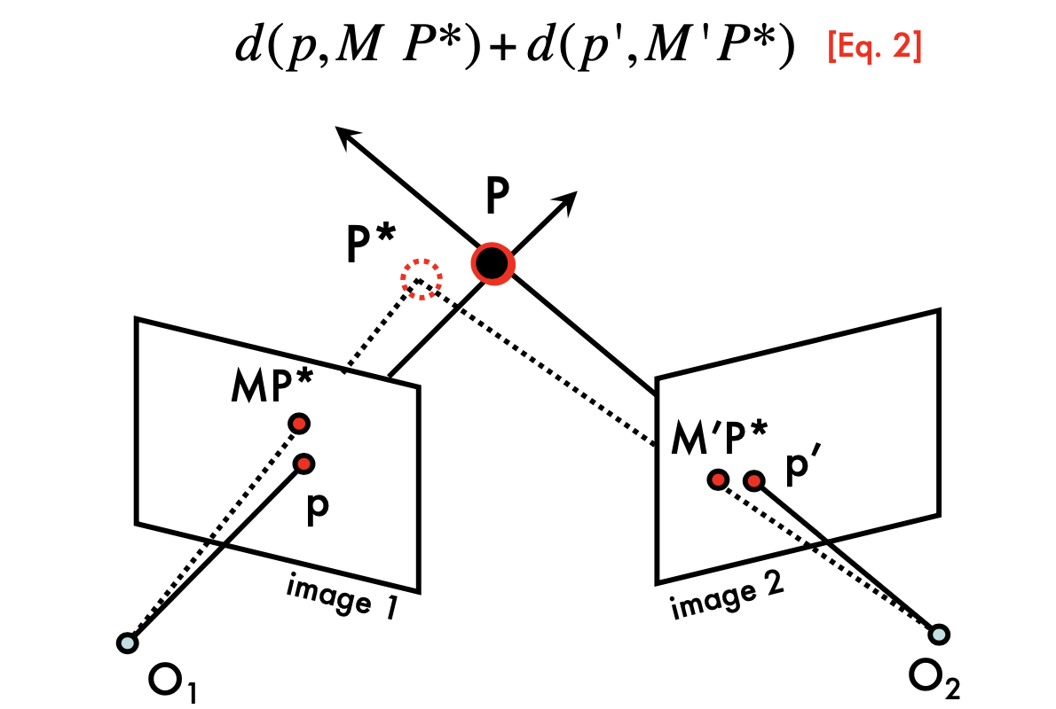
- find minimizes:
Triangulation:
- P* is the estimation of actual P (P in 3D)
- Do not need to calculate the line in 3D, which is hard to do
Multi-view genometry
in this lecture, we suppose the corresponding p and p' is given
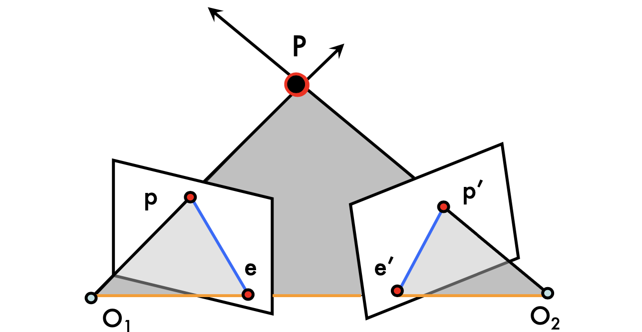
the line connect O1 and O2 is called baseline
Epipolar lines: blue lines, p'e' and pe
Epipoles: e, e'
= intersections of baseline with image planes
= projections of the other camera center
Can we know where is p'?
- p' must be on epipolar line
- p' is no longer on the arbirarly position of the line
camera is canonical:
- K is identity matrix (K is the camera intrincs)
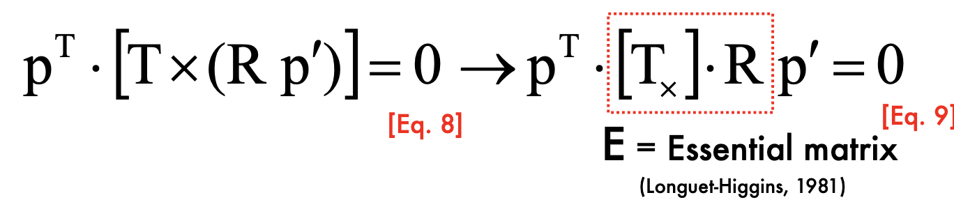
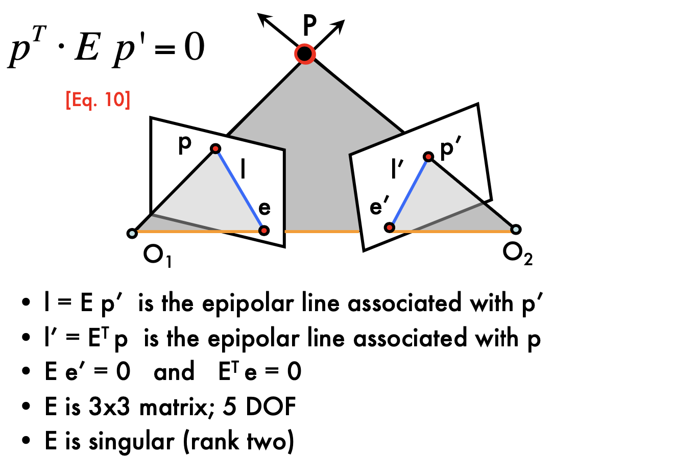
Epipolar Constraint:
- Essential Matrix
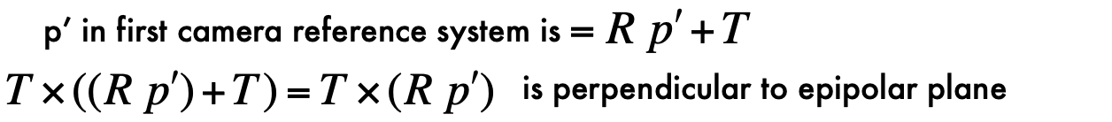
- p' is at the second camera reference system
is defined by p' and the base line, so must be associate with p' - E has 5 DOF: E is up to scale, and T has 3 DOF, and R has 3 DOF
Cross product to matrix:
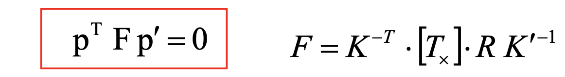
Fundamental Matrix:
- Esstential matrix is derived using canonical cameras assumption. Fundamental matrix does NOT have this assumption

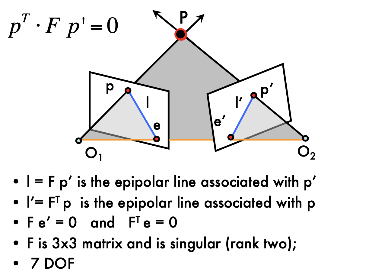
- can also be calcualted according to just observations
- F gives constrains on how the scene changes under view point transformations
Estimating F
- 8 points algorithm:
- Step1:
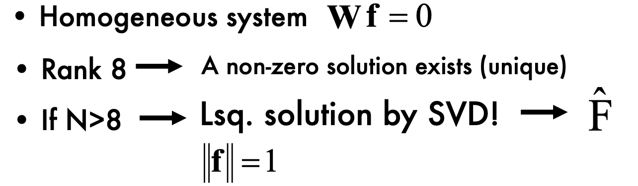
- Step2:
- Step1:
- What is the problem of 8-points algorithms
- uv in matrix W may be very large,some item in matrix W can be very small
- Highly un-balanced (not well conditioned)
- Values of W must have similar magnitude
- This creates problems during the SVD decomposition
- 8 points algorithm:
Normalized 8 points
- Mean square distance of the image points from origin is ~2 pixels

Lec6 Stereo Systems/ Multi-view Geometry
Essential Matrix
- camera are caronicol
- l = Ep
- pEp' = 0
- E = [Tx] R
Fundamental Matrix
Parallel image planes:


- Rectification: making two images "parallel"
- make triangulation easy
- rectification is a homography (projective transformation)
- Application: view morphing
- New views can be synthesized by linear interpolation
Parallel image planes
- O1-xyz are attached to the camera
- p and p' share same v coordinates (parallel)
- Rectification: make any two images parallel, homographic transformation H
- homographic transformation ??: transfrom a plan to another plane
- homographic transformation ??: transfrom a plan to another plane
- Inteplate view between two parallel images -> get different views
Why are parallel images important?
Makes triangulation easy - point triangulation
disparity = p_u - p_u', propotional to B*f/z
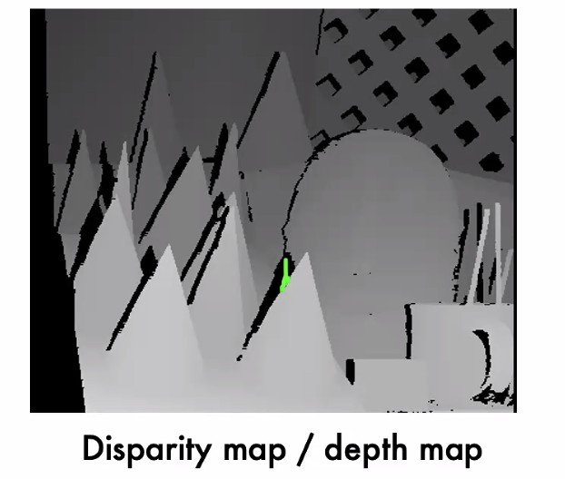
the black points are not shadows, are occlusions(do not how to decided)
Make the correspondence problem easier
Correspondence problem
- p belongs to l = Fp' => 1 dimensional search problem
- What's the problem?
- different lighting?
Window-based correlation Methods
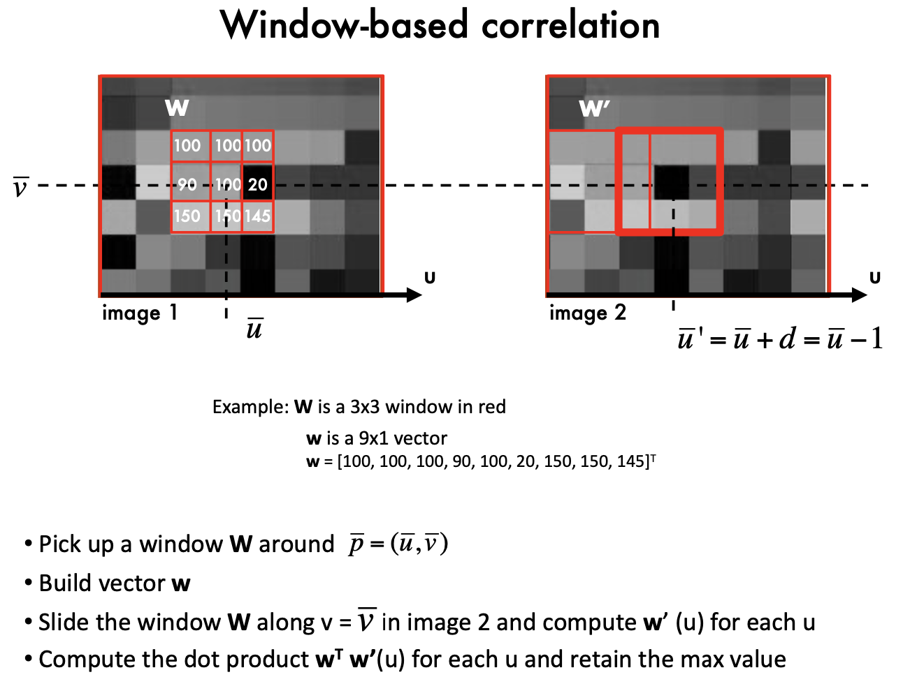
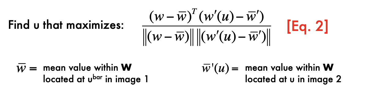
nomalize: Changes in the mean and the variance of intensity values in corresponding windows!
Effect of the window size
Smaller window
More detail
More noise
Larger window
Smoother disparity maps
Less prone to noise
Issues of Corresponence problem:
- Fore shortening effect
- Oclusions
- To reduce the effect of foreshortening and occlusions, it is desirable to have small B / z ratio!
- However, when B/z is small, small errors in measurements imply large error in estimating depth
Base line trade-off:
- Small errors in measure ments imply large error in estimating depth; small B/z ratio brings large triangulation error when measurement error

- Small errors in measure ments imply large error in estimating depth; small B/z ratio brings large triangulation error when measurement error
Non-local constraints to help enforce the correspondence
Difficult:
- Occlusions - Fore shortening - Baseline trade-off - Homogeneous regions
- Repetitive patterns
uniqueness: For any point in one image, there should be at most one matching point in the other image
Ordering: Corresponding points should be in the same order in both views
Smoothness: Disparity is typically a smooth function of x (except in occluding boundaries)
Multi-view Problem
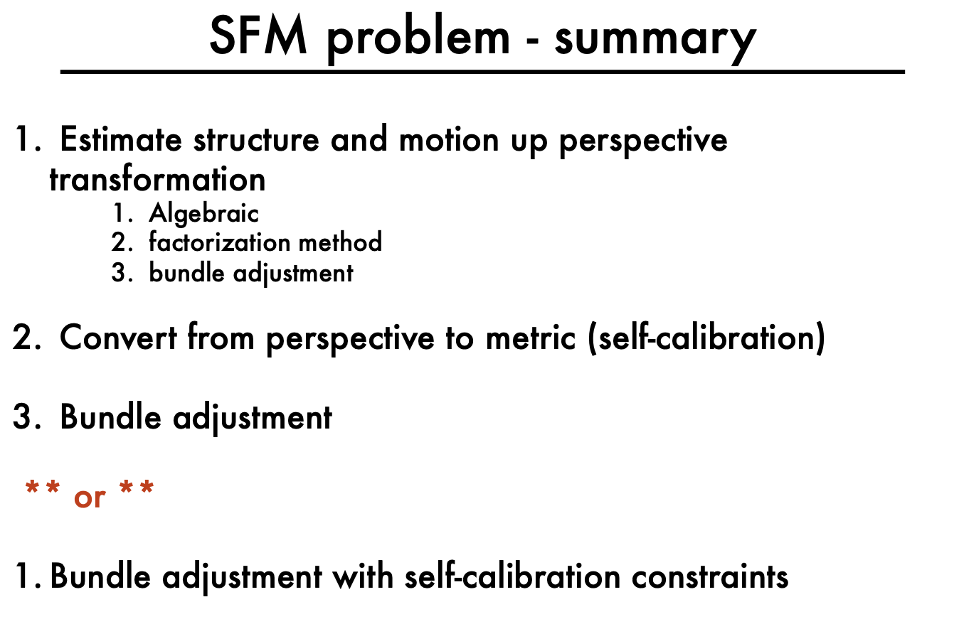
- Structure from motion problem (SFM): locolize the location of camera for each image; build 3D points
SFM:
- Affine SFM: Affine structure from motion
- Two approaches:
- Algebraic approach (affine epipolar geometry; estimate F; cameras; points)
- Factorization method
- Affine SFM: Affine structure from motion


Lec7 Multi-view Geometry
Affine SFM
Affine Structure-from-Motion Problem
Factorization method
- centering each image.
- Centering: subtract the centroid of the image points
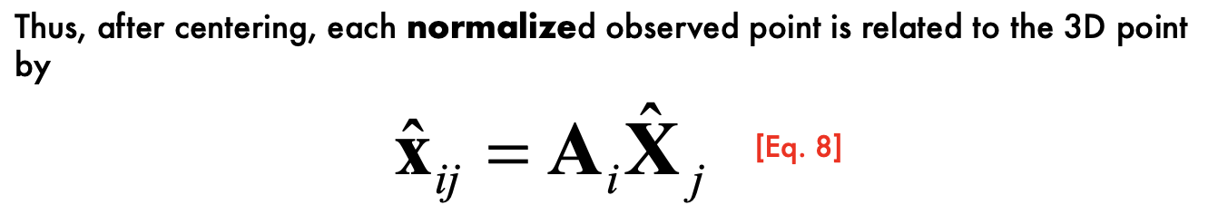
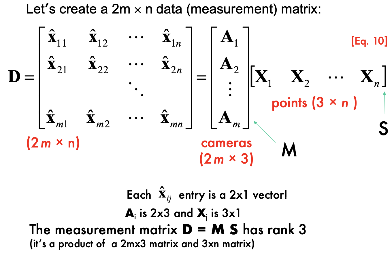
- SVD decomposition, and get combination of u and w is Motion(M), v is
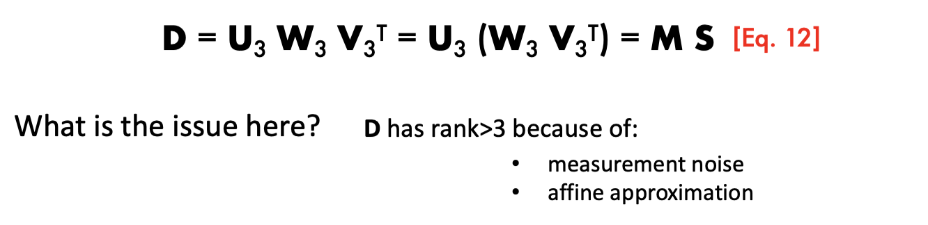
- Noises
- Affine approximation
Problems: Affine Ambiguity
The decomposition is not unique. We get the same D by applying the transformations: H is arbitrary 3*3 matrix describing an affine transformation
M* = M H
S* = H ^-1 S
Need additional constraints
The scene is determined by the images only up a similarity
transformation (rotation, translation and scaling)
- The ambiguity exists even for (intrinsically) calibrated cameras
- For calibrated cameras, the similarity ambiguity is the only ambiguity
Perspective SFM
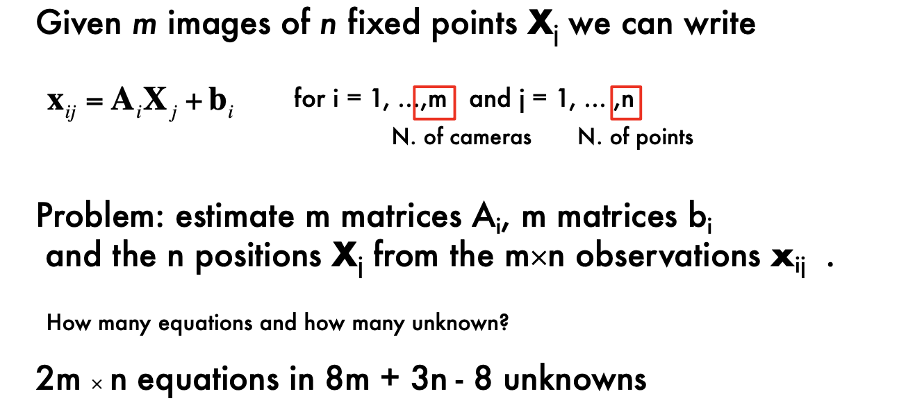
From the mxn observations x_ij, estimate:
m projection matrices M= motion i
n 3D points X_j = structure
Perspective SFM

- If the cameras are not calibrated, cameras and points can only be recovered up to a 4x4 projective (where the 4x4 projective is defined up to scale)
- projective ambiguity
- 2mn equations in 11m+3n – 15 unknowns
Methods:
algebraic approach
Factorization method - Affine SFM
Bundle adjustment
Algebraic Approach:
Compute the fundamental matrix F from two views
- at least 8 point correspondences, compute F
Use F to estimate projective cameras
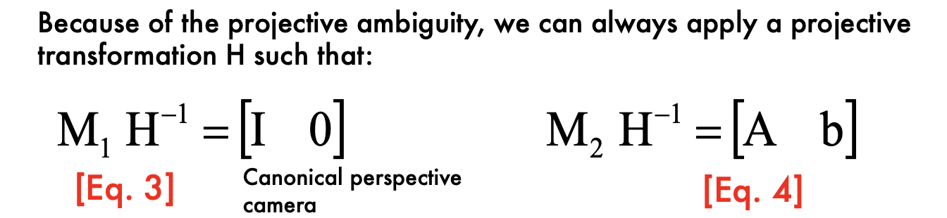
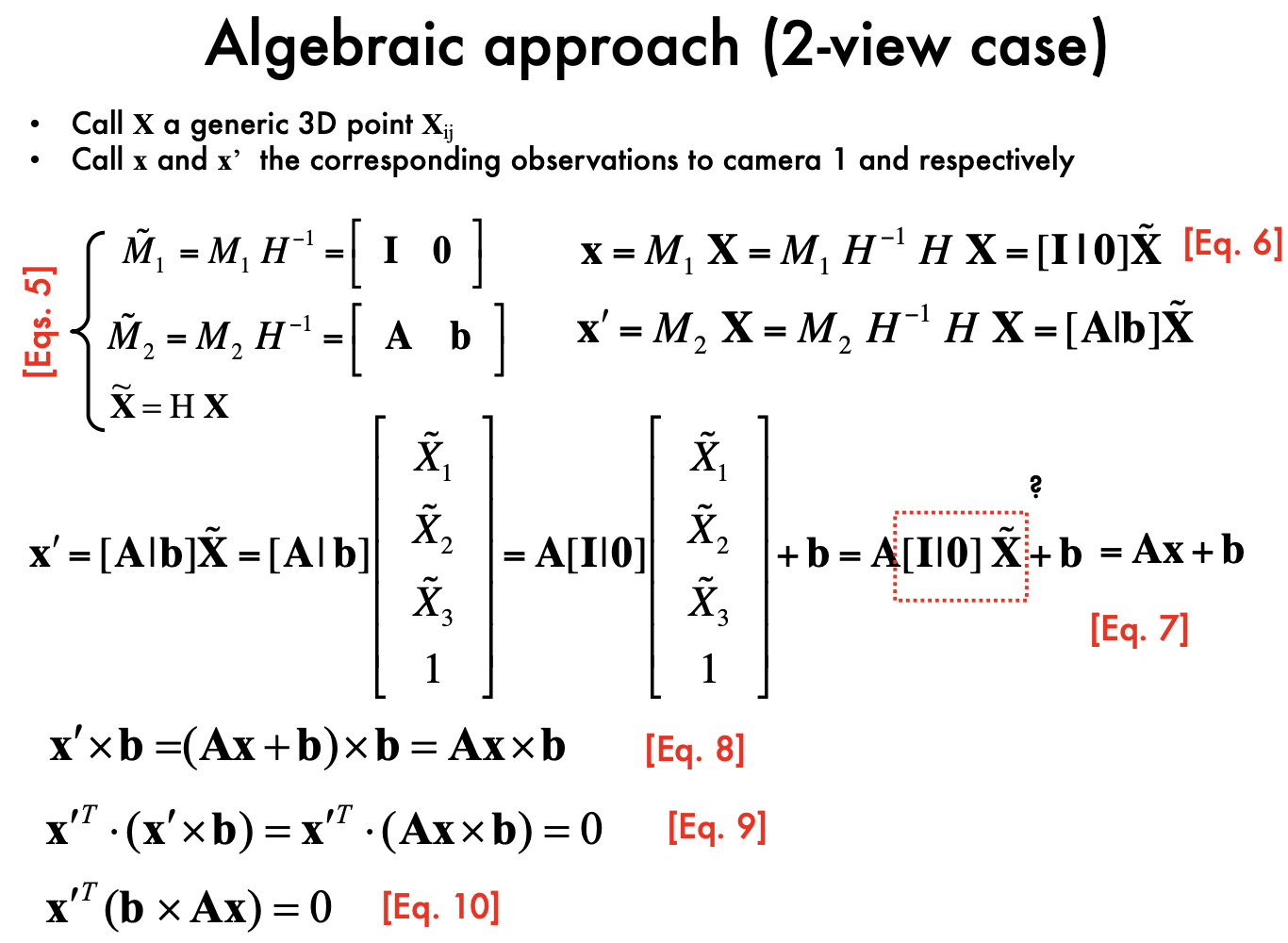
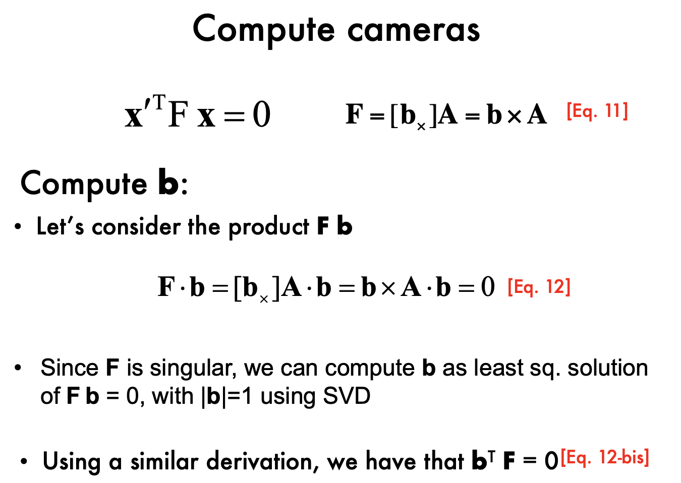
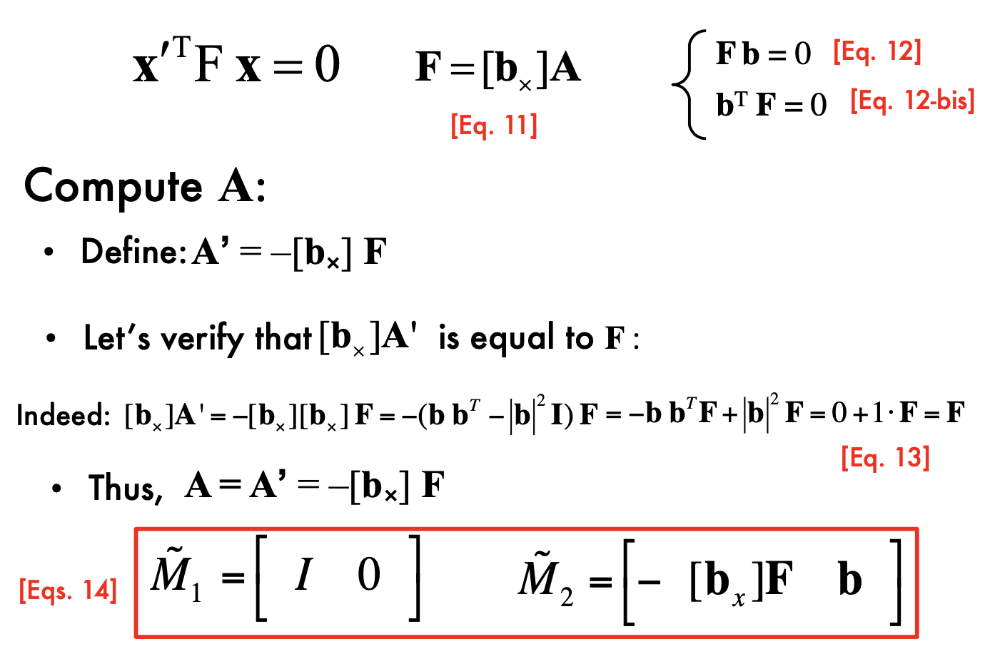
b is an epipole!
Use these cameras to triangulate and estimate points in 3D
- 3D points can be computed from camera matrices via SVD
Algebraic Approach: the N-views case
- Pairwise solutions may be combined together using bundle adjustment
Bundle adjustment
limitations of previous methods:
Factorization methods assume all points are visible. This not true if:
• occlusions occur • failure in establishing correspondences
Algebraic methods work with 2 views
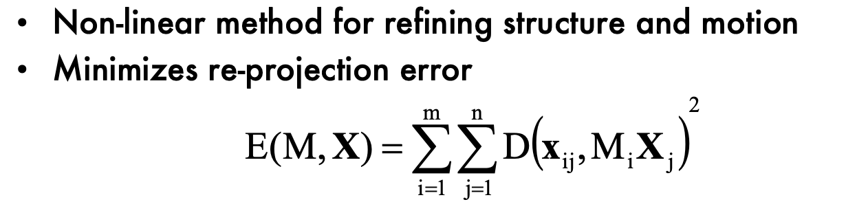
Use Levenberge-Marquardt Algorithm to minimize
Advantages:
- handle large number of views
- Handle missing data
Self-calibartion
the problem of recovering the metric reconstruction from the perspective (or affine) reconstruction
Several approaches:
- - Use single-view metrology constraints (lecture 4)
- - Direct approach (Kruppa Eqs) for 2 views
- - Algebraic approach
- - Stratified approach
Inject information about the camera during the bundle adjustment optimization
For calibrated cameras, the similarity ambiguity is the only ambiguity
 Projective reconstruction => affine reconstruction (up to affinity) => similarity reconstruction (up to scale)
Lec8 Active stereo & Volumetric stereo
Traditional Stereo
- Main problem: need to find correspondence
Replace one of the two cameras by a projector
- Projector geometry calibrated
- What’s the advantage of having the projector? Correspondence problem solved!
- Projector and camera are parallel
Laser Scanning:
- Optical triangulation
- Project a single stripe of laser light
- Scan it across the surface of the object
- This is a very precise version of structured light scanning
- Cons:
- slow
- Cannot capture deformations in time
Active stereo
- - Dense reconstruction - Correspondence problem again - Get around it by using color codes
Depth sensing
- Infrared laser projector combined with a CMOS sensor
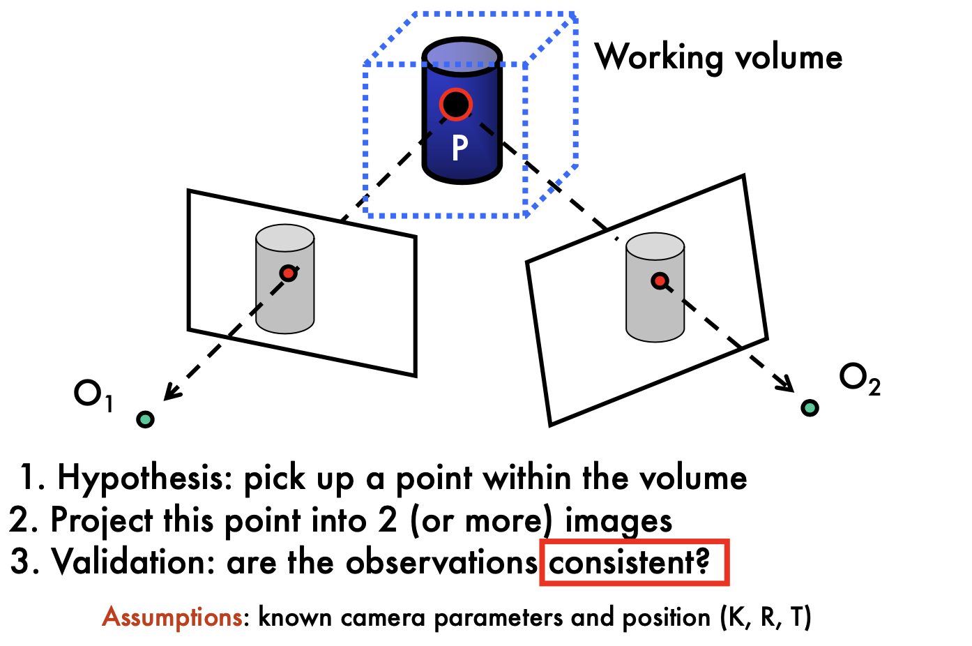
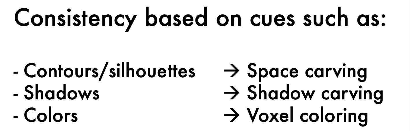
Volumetric stereo:
Contours / silhouettes
silhouette is defined as the area enclosed by the apparent contours
Using contours/silhouettes in volumetric stereo, also called
space carving
How to use Contours: visual hull / visual corn
Consistency: A voxel must be projected into a silhouette in each image
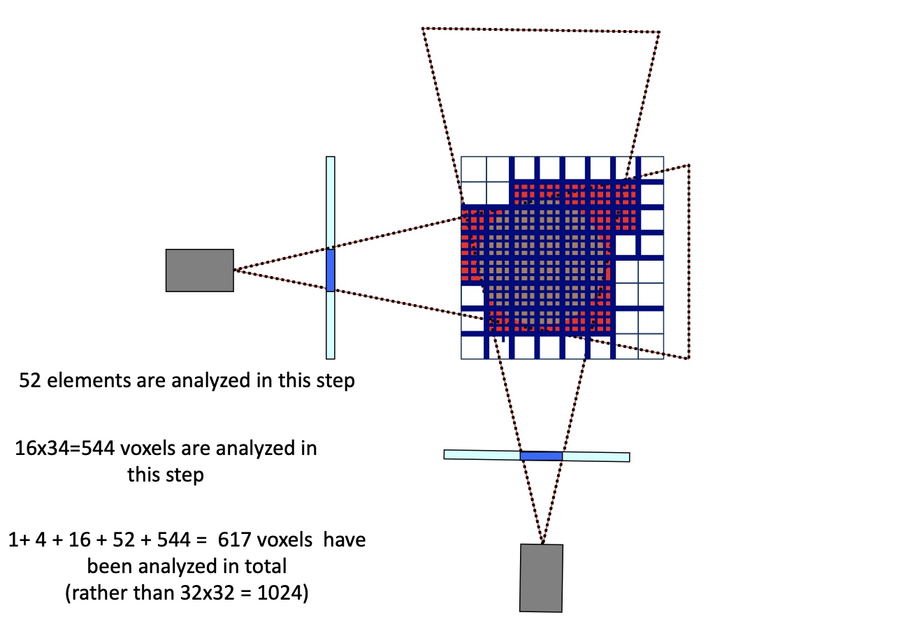
Space carving complexity: O(n3)
- use Octrees to speedup
pros and cons:
- Robust and simple
- No need to solve for correspondences
- Produce conservative estimates
- cons: Accuracy function of number of views
- cons: Concavities are not modeled
Space Carving:
- use contours / silhouettes
Shadow Carving
Self-shadows are visual cues for shape recovery
Camera + array of lights
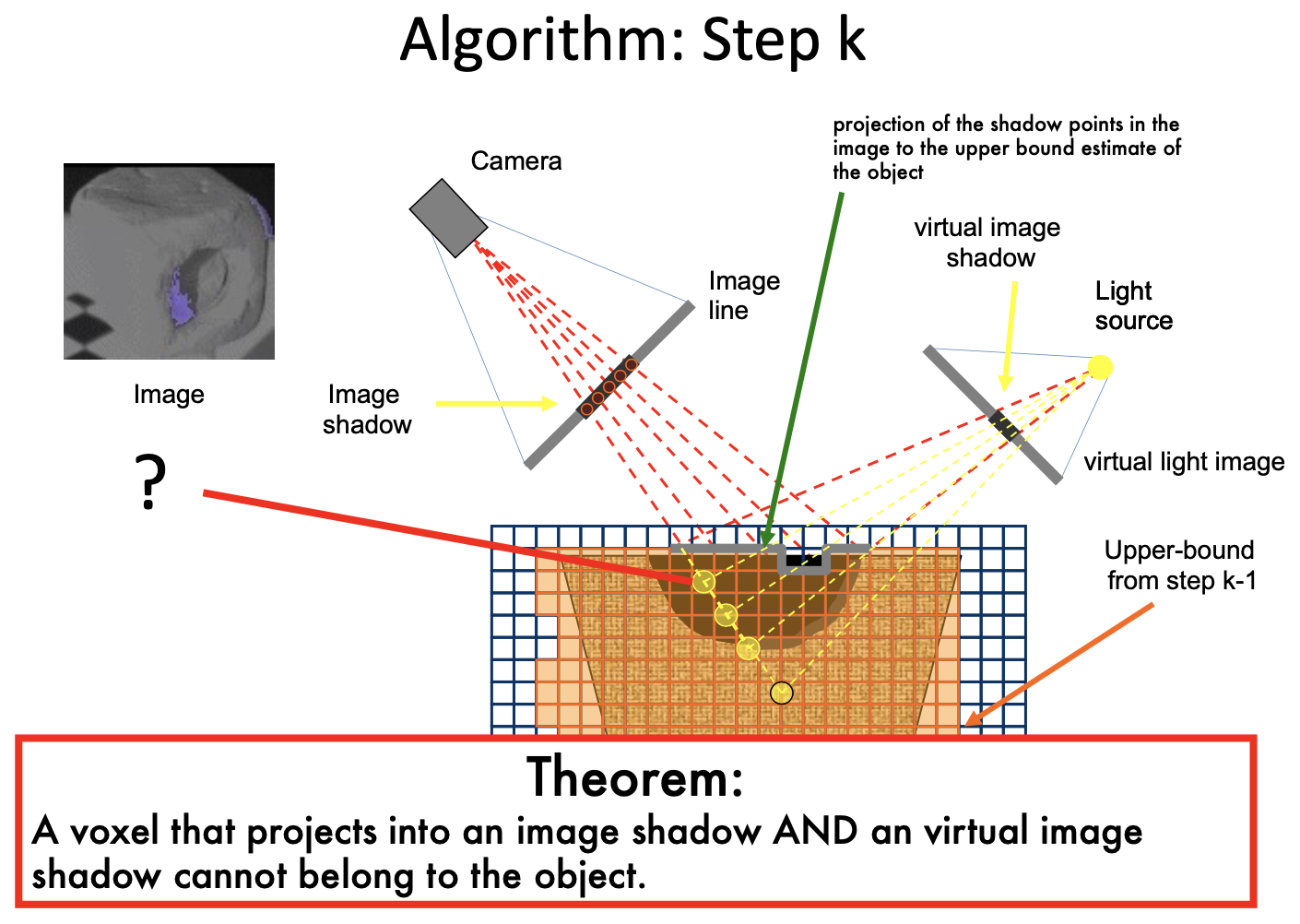
Summary:
- Produces a conservative volume estimate
- Accuracy depending on view point and light source number
- Limitations with reflective & low albedo regions
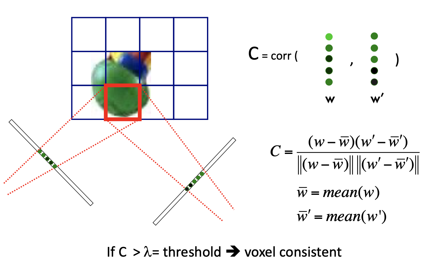
Voxel Coloring: use color as consistency test
- non-unique: multiple consistent scenes
- how to fix: need to use a visibility constraint
- if a voxel in two image are consistent, mark the voxel "in"
- A Critical Assumption: Lambertian Surfaces
- color is not related to the view point
- Photo consistency test
- Good things – Model intrinsic scene colors and texture – No assumptions on scene topology
- Limitations: – Constrained camera positions – Lambertian assumption
- non-unique: multiple consistent scenes
Lec9 Fitting and Matching
Fitting
- Choose a parametric model to fit a certain quantity from data
- Estimatemodelparameters
- Critical issues:
- noisy data
- outliers
- missing data (occlusion)
- Intra-class variation
- Techniques:
- least square methods
- RANSAC
- Hough Transform
- EM (Expectation Maximization)
Least square methods:

- h: the parameter of the model
- using calculus to solve
- Issue: fails completely for vertical lines, m is infinity
- Another way:


- rank deficient means a lot of solutions, not unique. Need an optimal solution
- using SVD to solve: last column of V correspond to the smallest singluar value
- Limitations: Robustness to noise is not good
RANSAC (RANdom SAmple Consensus)
Data elements are used to vote for one (or multiple) models
verify for a given model, see whether a good fit
Assumption 1: Noisy data points will not vote consistently for any single model (“few” outliers)
Assumption 2: There are enough data points to agree on a good model (“few” missing data)
is a fuction, P is a set of all data, I is a set of inlier, O is a set of Outlier Solve for
, residual is below threshold 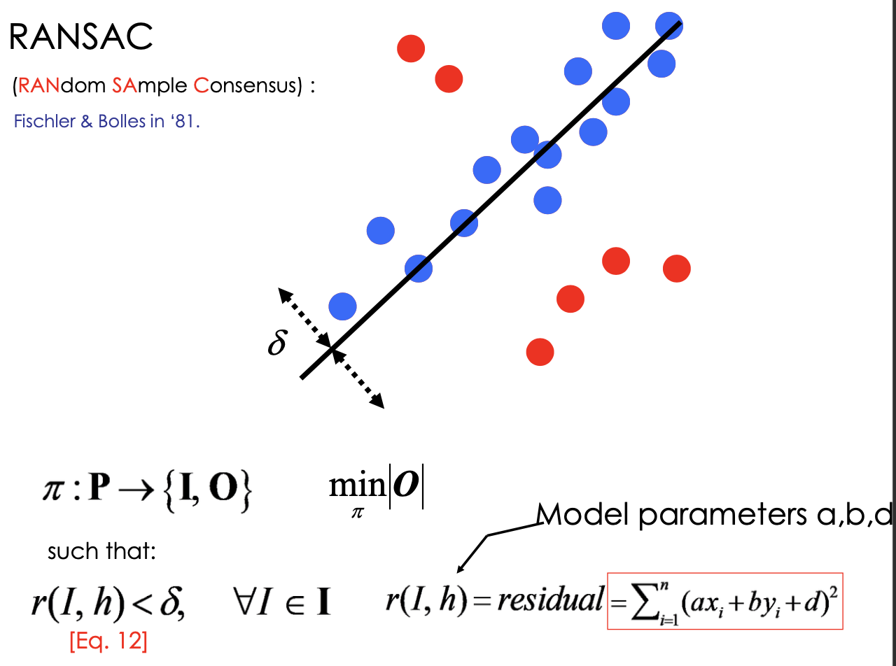
- need to decided threshold before run RANSAC
Algorithm:
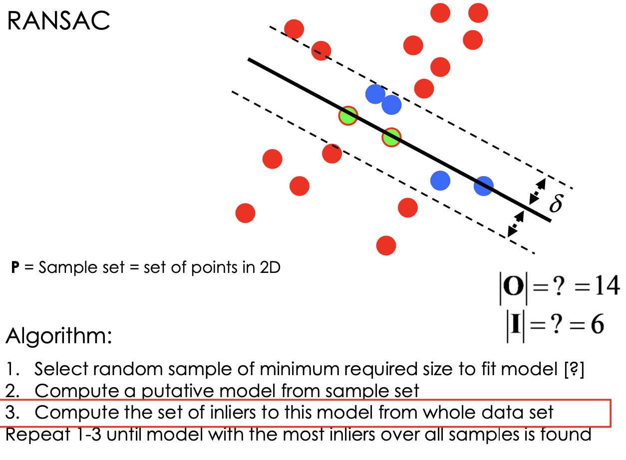
How many samples?
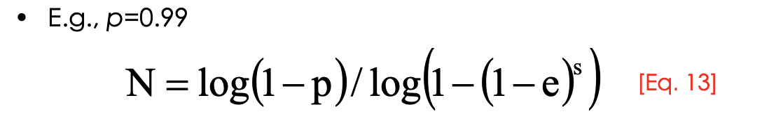
N samples are sufficient
N = number of samples required to ensure, with a probability p, that at least one random sample produces an inlier set that is free from “real” outliers
- want to get rid of outliers
number of sample is a function of s and e:
e = outlier ratio (make a guess)
s = minimum number of data points needed to fit the model (depend on number of parameters of model)
Usually, p=0.99
Good:
• Simple and easily implementable • Successful in different contexts
Bad:
• Many parameters to tune • Trade-off accuracy-vs-time • Cannot be used if ratio inliers/outliers is too small
Hough transforms
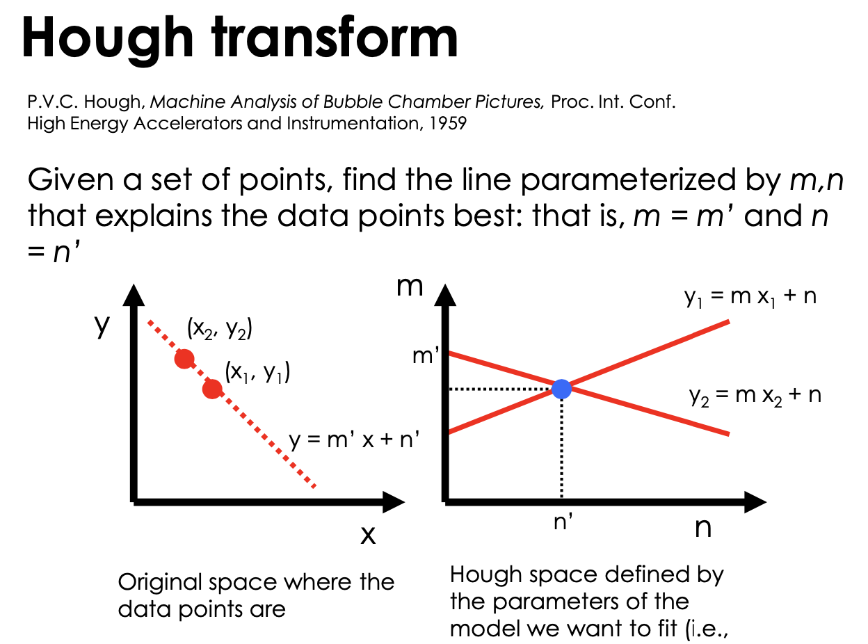
all points on x-y plane y =m'x + n' , result a intersection point in m-n plane
Issue: The parameter space [m,n] is unbounded...
- Use a polar representation for the parameter space
How to compute the intersection point? In presence of noise!
- IDEA: introduce a grid a count intersection points in each cell
- Issue: Grid size needs to be adjusted
Good:
• All points are processed independently, so can cope with occlusion/outliers
• Some robustness to noise: noise points unlikely to contribute consistently to any single cell
Bad:
• Spurious peaks due to uniform noise
• Trade-off noise-grid size (hard to find sweet point)
• Doesn’t handle well high dimensional models
Generalized Hough Transform
- Parameterize a shape by measuring the location of its parts and shape centroid
- Given a set of measurements, cast a vote in the Hough (parameter) space
Multi-model Fitting
- Incremental line fitting
- Hough transform
Fitting helps matching

- Fitting an homography H (by RANSAC) mapping features from images 1 to 2
- Bad matches will be labeled as outliers (hence rejected)!
- Application: Panoramas
Lec10 Representations and Representation Learning
What is a state? What is a representation?
- Markov Model
- State
- control input
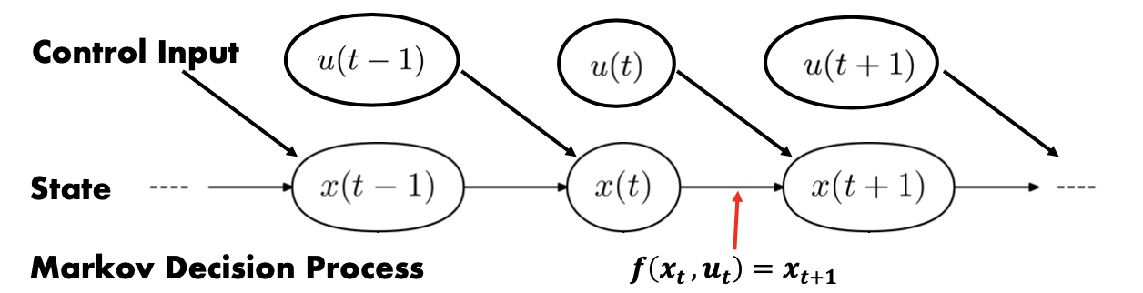
- State is partial or can not observable
-
-
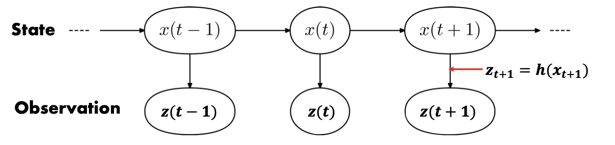
- Partially observable Markov decision process: Infer state x using observation z
- eg: 6DOF estimation
- Use observation go back to the state:
- Method1, eg: generative observation Model
- generative model: 𝑧 = h(𝑥)
- The relationship between x and z: 𝑃(𝑧|𝑥)
- generate z from x, then compare with ground truth
- Method2, eg: Discriminative observation Model
- Discriminative Model: 𝑧 = 𝑔(𝐼)
- The relationship between x and z: 𝑧 = 𝑥 = h(𝑥)
- h is filtering, take accumulative information from other frames
- Traking by decision
- Method1, eg: generative observation Model
Representation in Computer Vision
Requirements for Good Representations
- Compact (minimal)
- Explanatory (sufficient)
- Disentangled (independent factors)
- Hierarchical (feature reuse)
- Makes subsequent problem easier
object => representation => Mathematical Model(eg, classifier) => different types
Traditional Components:
- Color Histograms
- Model based Shapes
- Deformable Part based Models (DPM)
- Histogram of Gradients (HOG)
undertanding representations through low-dimensional embeddings
- t-SNE
nsupervised Representation Learning
- Auto-endcoder
- Reconstruction loss to minimize by finding optimal F
- Auto-endcoder
Representation Learning:
Reinforcement Learning (Cherry) Predicting a scalar reward given once in a while A few bits for some samples
Supervised Learning (Chocolate Coat)
Predicting category or vector of scalars per input as provided by human labels. 10-10k bits per sample
Unsupervised / Self-Supervised Learning (Cake)
Predicting parts of observed input or predicting future observations or events Millions of bits per sample
Summary
- State: Quantity that describes the most important aspect of a dynamical system at time t
- Representation: data format of input or output including a low-dimensional representation of sensor data
- Learned versus interpretable representations
- Visualize learned representations
- How to learn representations?
- Supervised
- Unsupervised
- Self-supervised